Calculus for Systems Modeling Archives - Page 9 of 11 - Sustainable Catalyst | Open Knowledge Lab for Ethical Strategy and Systems Intelligence

Archival mathematical workspace with transformed shaded-area graphs, flowing transparent channels, warped surfaces, layered accumulation models, notebooks, drafting tools, and pinned diagrams representing substitution and transformed accumulation.

Substitution and Transformations of Accumulation: How Calculus Rewrites System Change

Substitution and transformations of accumulation explain how accumulated meaning is preserved when a model changes variables, scales, coordinates, clocks, or state representations. This article treats substitution as a modeling principle rather than only a symbolic integration technique. It shows why transformed bounds, scale factors, differentials, orientation, monotonicity, and unit consistency matter when interpreting rates, densities, exposure, cost, distance, process time, normalized states, and transformed coordinates. In systems modeling, substitution helps prevent errors that arise when a convenient variable change silently alters what is being accumulated. The article also clarifies why nonmonotonic transformations may require piecewise treatment, why signed rates and nonnegative densities behave differently, and why transformed accumulation should be checked against the original representation whenever possible. The larger lesson is that changing variables is never merely algebraic; it changes the audit trail of accumulation and responsible model interpretation.

Archival systems modeling workspace with shaded accumulation graphs, flowing water, rising cumulative forms, notebooks, transparent overlays, stacked blocks, and drafting tools representing the Fundamental Theorem of Calculus.

The Fundamental Theorem of Calculus: Connecting Rates, Accumulation, and Change

The Fundamental Theorem of Calculus connects rates, accumulation, and net change, making it one of the central bridges between local behavior and system-level consequence. This article explains the theorem as a modeling principle rather than only a computational rule. It shows how accumulated rates correspond to endpoint differences, how accumulation functions recover local rates, and why state trajectories must be interpreted alongside intervals, baselines, sign conventions, and units. In systems modeling, the theorem clarifies how flows change stocks, how marginal quantities accumulate into totals, and how cumulative curves reveal underlying rates. It also shows why numerical approximation, measurement error, missing flows, and coarse time grids can create residuals between modeled rates and observed state changes. The theorem becomes a practical consistency test for interpreting continuous change responsibly across dynamic systems and for distinguishing net change from total activity claims.

Archival systems modeling workspace with shaded area graphs, cumulative bars, flowing water, reservoir levels, layered sediment diagrams, balances, notebooks, and drafting tools representing definite integrals and total change.

Definite Integrals and Total Change: How Calculus Measures Accumulated System Behavior

Definite integrals measure total change accumulated over an interval. This article develops definite integrals as a systems-modeling tool for cumulative emissions, total exposure, net flow, aggregate burden, distance traveled, work performed, energy transferred, total cost, and accumulated change in system state. It explains signed accumulation, net change, area under a curve, Riemann sums, interval boundaries, orientation, units, net change versus total variation, numerical approximation, uncertainty, and responsible interpretation. The article emphasizes that definite integrals translate local rates, densities, intensities, and marginal quantities into interval-based totals only when the integrand, bounds, sign convention, units, and method are documented. Companion workflows in Python, R, SQL, and Haskell include definite-integral audits, signed and absolute accumulation, interval records, unit checks, trapezoidal approximation, assumption registries, and advanced mathematical audit reports.

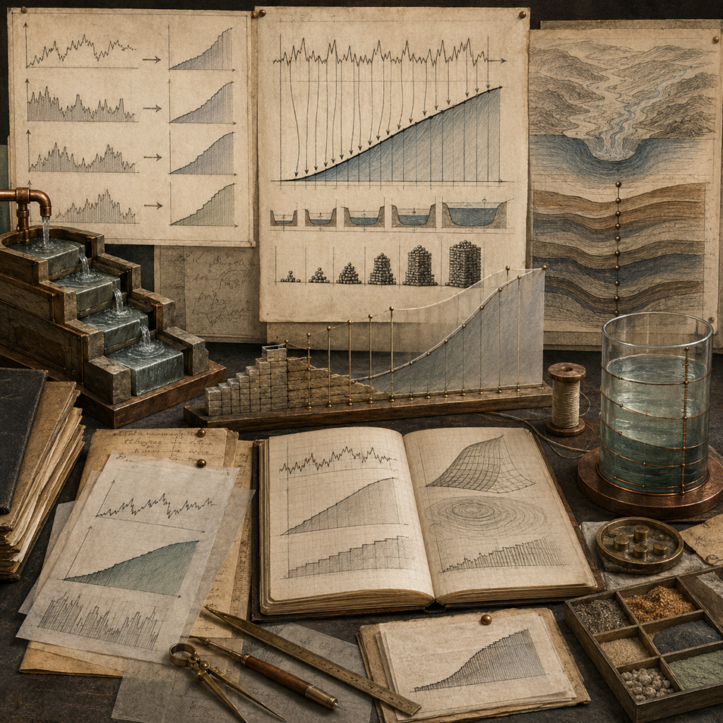
Vintage systems modeling workspace with stepped water channels, cumulative graphs, shaded areas, rising stacks, layered sediment diagrams, notebooks, measuring tools, and a glass reservoir representing antiderivatives and accumulation.

Antiderivatives and the Recovery of Accumulation: How Calculus Reconstructs System Change

Antiderivatives recover accumulated quantities from rates of change. This article develops antiderivatives as a systems-modeling tool for reconstructing stocks from flows, exposure from intensity, distance from velocity, burden from rate, cumulative cost from marginal cost, and system state from observed change. It explains primitive functions, constants of integration, initial conditions, flow-to-stock reasoning, marginal-to-total reasoning, unit consistency, numerical accumulation, reconstruction from data, calibration, uncertainty, and responsible interpretation. The article emphasizes that a rate alone does not determine an absolute quantity without a baseline, interval, domain, and accumulation assumption. Companion workflows in Python, R, SQL, and Haskell include antiderivative recovery audits, flow-to-stock reconstruction, trapezoidal accumulation, baseline records, typed accumulation structures, unit checks, assumption registries, and advanced mathematical audit reports for responsible recovery of accumulated system quantities across symbolic models, observed rate records, discrete time grids, and decision-relevant cumulative reporting workflows contexts.

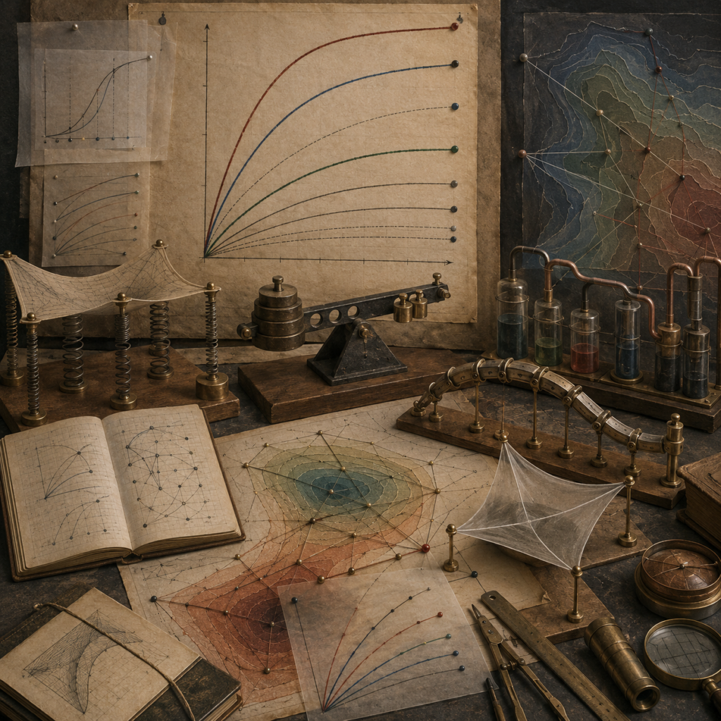
Vintage systems modeling workspace with response curves, flexible surface models, springs, weighted balances, contour maps, network diagrams, glass vessels, notebooks, and drafting tools representing elasticity, sensitivity, and marginal response.

Elasticity, Sensitivity, and Marginal Response: How Calculus Measures System Responsiveness

Elasticity, sensitivity, and marginal response describe how strongly a system reacts when an input, parameter, condition, or policy variable changes. This article develops these ideas as a bridge between derivative-based calculus and systems modeling, connecting marginal change, relative responsiveness, parameter dependence, local and global sensitivity, scaling, units, nonlinear response, decision thresholds, numerical estimation, uncertainty, and responsible interpretation. It explains why the same absolute change can be minor at one scale and decisive at another, why local responsiveness depends on operating point, and why sensitivity should be documented before model conclusions are treated as stable. Companion workflows in Python, R, SQL, and Haskell include elasticity audits, marginal-response diagnostics, finite-difference checks, normalized parameter sensitivity, baseline records, typed sensitivity structures, assumption registries, domain warnings, and advanced mathematical audit reports for robust interpretation.

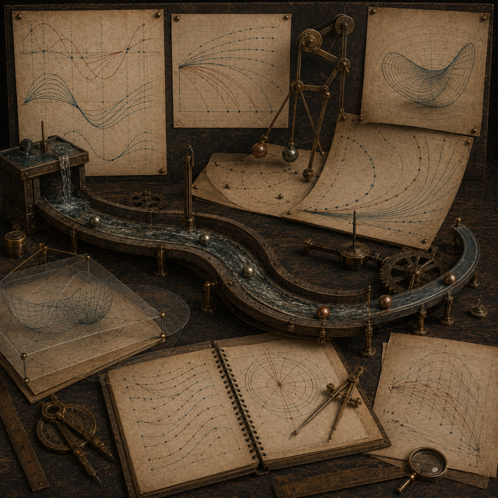
Vintage systems modeling workspace with curved tracks, moving spheres, pendulum mechanisms, layered curve diagrams, surface models, notebooks, and drafting tools representing second derivatives, curvature, and acceleration.

Second Derivatives, Curvature, and Acceleration: How Calculus Reveals Changing System Behavior

Second derivatives describe how change itself changes. This article develops second derivatives as a systems-modeling tool for acceleration, concavity, curvature, inflection, marginal change, nonlinear response, second-order approximation, optimization, stability interpretation, numerical estimation, and responsible interpretation. It explains how a system can increase while growth slows, decline while collapse accelerates, or appear locally stable while curvature reveals emerging pressure. Examples include population growth, infrastructure congestion, climate pathways, epidemiological curves, economic margins, and machine-learning objectives. Companion workflows in Python, R, SQL, and Haskell include second-derivative audits, curvature diagnostics, acceleration interpretation, concavity classification, inflection-candidate review, finite-difference checks, typed curvature records, assumption registries, noise and step-size warnings, and advanced mathematical audit reports for responsible interpretation of curvature-based claims across nonlinear, noisy, and finite-precision systems.

Vintage systems modeling workshop with linked reservoirs, flowing channels, pulleys, pendulum mechanisms, gears, layered diagrams, notebooks, and drafting tools representing related rates and interdependent motion.

Related Rates and Interdependent Motion: How Calculus Tracks Connected System Change

Related rates explain how one rate of change is linked to another when system variables move together under a shared relationship. This article develops related rates as the calculus of interdependent motion, connecting time-dependent variables, differentiated constraints, the chain rule, implicit differentiation, tangent-space motion, units, measurement error, numerical derivatives, and systems interpretation. It shows how reservoir height implies volume change, infrastructure load and capacity determine utilization motion, epidemiological flows shift prevalence, environmental emissions affect concentration, economic variables move through product and quotient structures, and feature drift propagates through computational pipelines. Companion workflows in Python, R, SQL, and Haskell include related-rates audits, interdependent-motion diagnostics, finite-difference checks, operating-point records, unit review, typed rate relationships, assumption registries, conditioning warnings, and advanced mathematical audit reports for responsible interpretation of linked rates across noisy observations, constrained relationships, local operating points, and finite-precision workflows today.

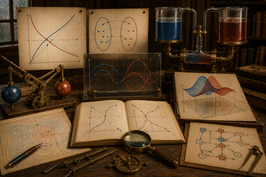
Vintage scientific modeling studio with paired curves, mirrored mappings, linked fluid vessels, mechanical arms, surface diagrams, contour maps, notebooks, and drafting tools representing inverse functions and system interpretation.

Inverse Functions and System Interpretation: How Calculus Reverses Inputs, Outputs, and Meaning

Inverse functions turn systems modeling around by asking what input, state, parameter, pathway, or condition could have produced an observed output. This article develops inverse functions as both a formal calculus topic and a systems-interpretation tool for calibration, diagnosis, reconstruction, inverse problems, target-setting, and model explanation. It covers forward versus inverse thinking, one-to-one behavior, domain restrictions, inverse derivatives, the inverse function theorem, local and global inverses, identifiability, recoverability, conditioning, stability, branch selection, and interpretive ambiguity. Examples include environmental reconstruction, epidemiological parameter recovery, infrastructure sensing, policy target-setting, calibration, and machine-learning interpretation. Companion workflows in Python, R, SQL, and Haskell include inverse interpretation audits, forward checks, recoverability diagnostics, derivative-based sensitivity, domain review, typed inverse records, assumption registries, conditioning warnings, and advanced mathematical audit reports for responsible inverse reasoning across noisy observations, constrained domains, branch-specific assumptions, calibration uncertainty, and finite-precision computational workflows.

Archival mathematical modeling workspace with paired vessels, coupled curves, contour diagrams, intersecting surfaces, mechanical linkages, notebooks, and drafting tools representing implicit differentiation and coupled relationships.

Implicit Differentiation and Coupled Relationships: How Calculus Tracks Linked System Change

Implicit differentiation explains how coupled variables co-adjust when a constraint, equilibrium condition, conservation law, feasibility boundary, or feedback relationship must remain true. This article develops implicit differentiation as both a formal calculus technique and a systems-modeling tool for relationships that cannot honestly be reduced to a simple explicit function. It covers explicit versus implicit models, total differentials, constraint motion, the implicit function theorem, coupled variables, equilibrium sensitivity, feedback co-adjustment, systems of equations, Jacobian formulations, singular cases, and loss of local solvability. Examples include market equilibrium, resource-population coupling, infrastructure utilization, epidemiological thresholds, climate balance conditions, calibration, and inverse problems. Companion workflows in Python, R, SQL, and Haskell include implicit sensitivity audits, finite-difference checks, regularity-condition review, typed coupled records, assumption registries, Jacobian conditioning warnings, and advanced mathematical audit reports for responsible interpretation of constrained, coupled, equilibrium-based system relationships.