
Last Updated June 28, 2026
Calculus for Systems Modeling examines how continuous change, accumulation, approximation, optimization, feedback, and dynamic interaction can be represented mathematically across ecology, economics, infrastructure, climate, engineering, epidemiology, public policy, sustainability, and complex systems practice. Many real-world systems do not move only in discrete jumps. They grow, decline, accumulate, diffuse, oscillate, stabilize, destabilize, respond, interact, and reorganize through time and space. Calculus provides one of the core mathematical languages for describing these processes, while scientific-computing workflows make it possible to simulate, inspect, approximate, compare, and responsibly interpret them.
This article map treats calculus not merely as a classroom sequence of derivative and integral techniques, but as a modeling language for dynamic systems. Derivatives describe rates of change, marginal effects, sensitivity, acceleration, local system behavior, and feedback response. Integrals describe accumulation, exposure, total change, flow-to-stock reasoning, conserved quantities, cumulative burden, and long-run effects. Multivariable calculus extends these ideas into interacting systems, gradients, constraints, surfaces, local approximation, and high-dimensional model behavior. Vector calculus supports the study of spatial fields, flows, circulation, flux, diffusion, conservation, and boundary reasoning. Differential equations turn calculus into a language for systems whose current state depends on rates, feedback, forcing, coupling, memory, and initial conditions.
Because many real systems are nonlinear, partially observed, noisy, spatially distributed, parameter-sensitive, or computationally difficult, calculus for systems modeling must also be computational. Closed-form solutions remain important, but many useful models require numerical differentiation, numerical integration, finite differences, ordinary differential equation solvers, partial differential equation approximations, simulation, parameter sweeps, sensitivity analysis, symbolic computation, reproducible notebooks, typed model records, audit trails, and careful interpretation. This series therefore joins formal mathematics, systems modeling, scientific computing, and responsible judgment into a single framework for reasoning about continuous change.
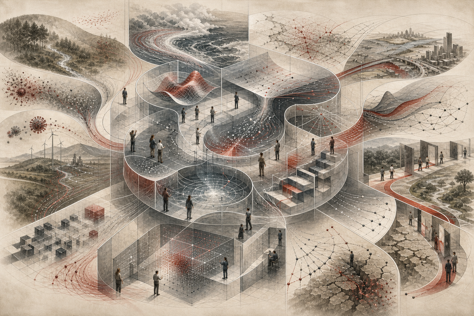
Calculus appears here not merely as a collection of techniques, but as a disciplined architecture for reasoning about change. It clarifies how systems move, how quantities accumulate, how local effects become global consequences, how feedback alters trajectories, how constraints shape optimization, and how spatial processes can be represented through fields and flows. In mathematical modeling, calculus helps transform dynamic phenomena into formal structures that can be analyzed, simulated, tested, revised, and communicated.
This matters because many systems studied across environmental science, economics, engineering, infrastructure analysis, epidemiology, sustainability, and public policy are fundamentally dynamic. Populations expand and contract. Temperatures shift in response to forcing and feedback. Resource stocks are depleted or replenished through time. Markets respond to marginal incentives. Built systems experience flow, decay, congestion, and capacity limits. Pollutants diffuse through air, water, and soil. Energy systems redistribute loads under changing demand. These are not static worlds. They are worlds of motion, accumulation, pressure, response, uncertainty, and interaction.
GitHub Repository
The companion repository for this article map is designed as a reproducible mathematical-modeling workspace. It contains article-level folders for calculus-based systems modeling, including symbolic reasoning, numerical approximation, dynamic simulation, differential-equation workflows, sensitivity analysis, parameter sweeps, typed model records, structured scenario data, reproducible notebooks, documentation, generated outputs, and governance-oriented review artifacts.
Complete Code Repository
Companion article folder with Python, R, Julia, SQL, Haskell, C, C++, Fortran, Rust, Go, notebooks, documentation, synthetic teaching data, generated outputs, schemas, and Canvas-ready workflow artifacts for calculus-based systems modeling, continuous-change analysis, accumulation, numerical approximation, dynamic simulation, sensitivity analysis, and responsible mathematical interpretation.
Calculus as the Mathematics of Change
Calculus begins from a simple but profound modeling problem: how can continuous change be represented with precision? Many systems are not adequately described by a single value at a single time. They unfold. They respond. They accumulate. They move through trajectories. They may approach equilibrium, diverge, oscillate, accelerate, slow down, cross thresholds, or shift into new regimes.
The derivative gives formal structure to local change. It describes how a quantity changes at or near a point. This makes it central to modeling growth, decay, acceleration, marginal response, sensitivity, and instantaneous rate. The integral gives formal structure to accumulation. It describes how local contributions gather into total change, total exposure, total mass, total cost, total energy, total flow, or total system burden.
Calculus also makes it possible to connect local and global reasoning. A derivative may describe local behavior, but the accumulation of local changes can produce system-level consequences. An integral may summarize cumulative effects, but those effects may depend on changing rates through time. Differential equations connect these ideas by representing systems in which the rate of change itself determines the path of the system.
For systems modeling, this is the central insight: dynamic systems are not only collections of quantities. They are structured relationships among quantities that change.
Why Calculus Matters for Systems Modeling
Many systems studied across environmental science, economics, engineering, infrastructure analysis, epidemiology, sustainability, and public policy are fundamentally dynamic. Populations expand and contract. Temperatures shift in response to forcing and feedback. Resource stocks are depleted or replenished through time. Markets respond to marginal incentives. Built systems experience flow, decay, congestion, and capacity limits. Pollutants diffuse through air, water, and soil. Energy systems redistribute loads under changing demand.
Calculus matters because it provides the formal language for representing these processes. Derivatives make it possible to analyze rates of change, marginal effects, sensitivity, acceleration, and local behavior. Integrals make it possible to analyze accumulation, total exposure, aggregate change, conserved quantities, and flow-to-stock reasoning. Multivariable calculus extends this logic to systems with interacting variables, constraints, gradients, and surfaces. Vector calculus introduces fields, flows, and conservation across space. Differential equations make it possible to represent systems whose present condition depends on ongoing motion, feedback, external forcing, and coupled dynamics.
For mathematical modeling, the importance of calculus is not only theoretical. Most real applications depend on approximation, numerical solution, simulation, visualization, and computational experimentation. Closed-form analytic solutions are often unavailable or insufficient. Real systems may be nonlinear, high-dimensional, partially observed, spatially distributed, or computationally intensive. For that reason, calculus must also be understood as a practical modeling discipline implemented through software, algorithms, and reproducible workflows.
Scope of This Content Pillar
This pillar is designed as a comprehensive treatment of calculus while remaining organized enough to support cumulative learning over time. It does not treat calculus merely as a classroom sequence of rules, nor merely as a programming tutorial. Instead, it treats the subject as a major intellectual and methodological foundation for mathematical modeling and systems modeling.
The series moves across several levels at once. At the mathematical level, it examines the conceptual and formal foundations of limits, continuity, differentiation, integration, multivariable analysis, sequences and series, vector calculus, optimization, and differential equations. At the interpretive level, it shows how these concepts clarify the behavior of dynamic systems, including growth, decay, accumulation, equilibrium, instability, diffusion, feedback, nonlinear change, spatial interaction, sensitivity, and regime change. At the computational level, it explores how calculus can be implemented through reproducible workflows in Python, R, Julia, SQL, Haskell, C, C++, Fortran, Rust, Go, notebooks, schemas, documentation, and generated outputs.
The goal is not simply to teach isolated techniques. It is to build a durable framework for understanding how continuous mathematics supports dynamic reasoning across domains such as climate systems, ecology, economics, infrastructure, engineering, epidemiology, sustainability, decision science, and data-driven scientific inquiry. The result is a series that is mathematical in rigor, systems-oriented in interpretation, and computational in practical orientation.
Mathematics and Computational Modeling Languages
A full treatment of calculus for systems modeling requires more than symbolic derivation alone. Mathematics establishes the conceptual structure, but computation makes it possible to investigate systems that are too complicated for purely analytic treatment. For that reason, this series is designed around formal mathematics, scientific computing, reproducible workflows, and multi-language implementation.
The mathematical dimension addresses the logic of continuous change itself. It asks what a limit means, what a derivative measures, what an integral accumulates, how continuity structures a model, how local approximation supports global reasoning, how fields encode distributed processes, and how differential equations express evolving states. This is the level at which concepts must be understood with precision.
The computational dimension extends that reasoning into systems modeling practice. Python supports numerical methods, symbolic computation, simulation, optimization, data pipelines, and scientific-computing workflows. R supports statistical integration, visualization, sensitivity analysis, reproducible reporting, and model comparison. Julia supports high-performance numerical modeling and differential-equation workflows. SQL supports structured model inputs, parameter registries, scenario tables, provenance records, and output governance. Haskell supports strongly typed functional representations of model states, assumptions, transformations, and validation logic. C, C++, and Fortran connect the series to performance-oriented scientific computing and legacy numerical methods. Rust and Go support reliable command-line tools, typed workflows, reproducible pipelines, and scalable modeling infrastructure. Notebooks and documentation connect these implementations to explanation, teaching, auditability, and interpretation.
Together, these languages are not included for novelty. They show that calculus-based systems modeling can be expressed at multiple levels: conceptual, analytical, statistical, numerical, typed, procedural, compiled, reproducible, and governance-oriented. The goal is not to turn every article into a programming survey, but to make the companion repository broad enough to support serious systems modeling practice.
Mathematical Lens
A derivative represents instantaneous or local change:
f'(x)=\lim_{h \to 0}\frac{f(x+h)-f(x)}{h}
\]
Interpretation: The derivative measures how a function changes near a point. In systems modeling, it can represent marginal response, growth rate, velocity, acceleration, sensitivity, or local system behavior.
An integral represents accumulation:
\int_a^b f(x)\,dx
\]
Interpretation: The integral accumulates local contributions across an interval. In applied modeling, it can represent total exposure, total flow, cumulative emissions, aggregate cost, accumulated energy, or total change.
The fundamental theorem of calculus connects rates and accumulation:
\int_a^b f'(x)\,dx=f(b)-f(a)
\]
Interpretation: The accumulated rate of change over an interval equals the net change in the underlying quantity. This connection is central to flow-to-stock reasoning.
A simple continuous-time dynamic model can be written as:
\frac{dx}{dt}=f(x,t,\theta)
\]
Interpretation: The state \(x\) changes through time according to a rule \(f\), which may depend on the current state, time, and parameters. This structure appears across population dynamics, climate systems, epidemiology, engineering, economics, and infrastructure modeling.
A multivariable system can be represented through partial derivatives:
\frac{\partial f}{\partial x_i}
\]
Interpretation: A partial derivative measures how a function changes with respect to one variable while others are held fixed. This is essential for modeling interacting variables and marginal effects in higher-dimensional systems.
A gradient collects partial derivatives into a vector of local change:
\nabla f=\left(\frac{\partial f}{\partial x_1},\frac{\partial f}{\partial x_2},\ldots,\frac{\partial f}{\partial x_n}\right)
\]
Interpretation: The gradient points in the direction of steepest increase. In modeling, it supports optimization, sensitivity analysis, spatial reasoning, and constrained decision problems.
A cumulative system stock can be modeled from a flow:
S(t)=S(0)+\int_0^t F(\tau)\,d\tau
\]
Interpretation: A stock at time \(t\) equals its initial value plus accumulated inflow or net flow over time. This structure appears in resource modeling, emissions accounting, epidemiology, infrastructure loading, and financial accumulation.
These formulas do not exhaust calculus. They show why calculus is central to systems modeling: it connects local change, cumulative consequence, spatial structure, dynamic behavior, and computational approximation.
Major Themes in Calculus for Systems Modeling
1. Continuous Change
Calculus begins from the insight that many important processes change continuously rather than only discretely. This theme includes limits, continuity, derivatives, local approximation, acceleration, and the interpretation of system motion through time. It is the conceptual basis for representing dynamic systems mathematically.
2. Accumulation and Aggregation
Integration makes it possible to move from local rates to cumulative quantities. This theme includes total change, stock formation, area and volume interpretation, cumulative exposure, conserved quantities, and flow-to-stock reasoning. In modeling practice, this is essential for resource accounting, environmental exposure, infrastructure loading, and long-run process analysis.
3. Optimization and Marginal Analysis
Many systems problems involve trade-offs, constraints, efficiency questions, or marginal response. Calculus provides tools for locating extrema, reasoning about slopes and sensitivity, and studying how local adjustments alter broader outcomes. This theme is especially important in economics, engineering, planning, and control.
4. Multivariable Interaction
Real systems rarely involve a single variable acting in isolation. Multivariable calculus makes it possible to study interacting variables, partial effects, gradients, directional change, Jacobians, Hessians, and constraint surfaces. This theme supports more realistic representations of coupled and interdependent processes.
5. Infinite Approximation
Calculus depends deeply on infinite processes. Sequences, series, convergence, and Taylor approximation allow functions to be represented, approximated, and analyzed when exact solutions are difficult or impossible. This theme links rigorous theory to practical numerical modeling.
6. Spatial Fields and Flow
When systems extend across space, vector calculus becomes indispensable. This theme includes vector fields, line integrals, surface integrals, divergence, curl, flux, and conservation across boundaries. It supports the study of transport, flow, circulation, and distributed systems.
7. Differential Equations and Dynamic Systems
Differential equations extend calculus into explicitly dynamic models whose present state depends on rates of change, feedback, forcing, and interaction. This theme includes first-order and higher-order equations, coupled systems, equilibrium, stability, oscillation, bifurcation, and nonlinear behavior.
8. Numerical Approximation and Simulation
Many meaningful calculus-based models cannot be solved exactly. Numerical approximation therefore becomes essential. This theme includes finite differences, numerical integration, iterative solvers, ordinary differential equation methods, computational stability, error analysis, and practical implementation across scientific-computing environments.
9. Interpretation and Model Judgment
Mathematical and computational outputs still require disciplined interpretation. This theme includes assumptions, boundary conditions, scaling, nondimensionalization, parameter sensitivity, model scope, uncertainty, and the distinction between elegant mathematics and credible applied reasoning.
Calculus and Modeling Judgment
Calculus gives modelers powerful formal tools, but it does not remove the need for judgment. Every calculus-based model depends on assumptions about continuity, differentiability, scale, boundary conditions, parameters, measurement, and system structure. A derivative may be mathematically well defined while being empirically difficult to estimate. An integral may produce a clean total while hiding uncertainty in the underlying rate. A differential equation may be elegant while omitting important feedbacks, thresholds, or social constraints.
For this reason, calculus for systems modeling must be joined to model assessment. Does the model represent the right scale? Are the variables meaningful? Are the parameters measurable? Do the assumptions match the phenomenon? Is a continuous model appropriate, or does the system contain discontinuities, shocks, thresholds, or discrete events that require a different representation? How sensitive are conclusions to numerical choices, boundary conditions, and parameter values?
A serious calculus-based modeling practice does not treat formalism as a guarantee of truth. It treats formalism as a disciplined way to reason, test, simulate, and revise. The strength of calculus lies not only in the formulas themselves, but in the interpretive discipline required to use them responsibly.
Calculus for Systems Modeling Article Map
The Calculus for Systems Modeling pillar is organized to move from foundations and single-variable calculus toward integration, approximation, multivariable analysis, vector calculus, differential equations, numerical methods, modeling interpretation, and applied systems case studies. The series is intentionally broad because calculus is not only one topic inside mathematical modeling. It is a central language for representing change, accumulation, sensitivity, optimization, flow, and dynamic behavior.
Part I. Foundations of Calculus
- What Is Calculus for Systems Modeling? — An opening article defining calculus as a formal language for modeling continuous change, accumulation, and dynamic behavior.
- Functions, Variables, and Mathematical Representation — A foundation for understanding how relationships among quantities become formal models.
- Domains, Ranges, and the Structure of Functional Models — An article on what inputs are valid, what outputs are meaningful, and how model boundaries shape interpretation.
- Infinity, Infinitesimals, and the Historical Problem of Change — A historical and conceptual treatment of how calculus emerged from the problem of motion and change.
- Limits and the Formal Basis of Calculus — A rigorous introduction to limits as the foundation of derivatives, integrals, continuity, and approximation.
- Continuity, Discontinuity, and Structural Breaks — A modeling article on when continuous assumptions are appropriate and when systems contain breaks, shocks, or thresholds.
- Differentiability and Local Behavior — A treatment of local smoothness, tangent behavior, and the conditions under which rate-based reasoning works.
Part II. Differentiation and Rates of Change
- Derivatives and Rates of Change — A core article on derivatives as the language of local change, marginal response, and instantaneous dynamics.
- Rules of Differentiation and Model Structure — An article on how derivative rules reflect structural relationships among modeled quantities.
- The Product Rule and Interaction Effects — A modeling interpretation of changing products, coupled quantities, and interaction terms.
- The Quotient Rule and Relative Change — A treatment of ratios, rates, efficiency measures, and relative system behavior.
- The Chain Rule and Composite Change in Interacting Systems — An article on nested change, mediated effects, and linked transformations across system layers.
- Implicit Differentiation and Coupled Relationships — A study of systems where variables are linked through constraints rather than explicit functions.
- Inverse Functions and System Interpretation — An article on reversing relationships, interpreting inputs from outputs, and model invertibility.
- Related Rates and Interdependent Motion — A systems article on multiple quantities changing together through shared constraints.
- Second Derivatives, Curvature, and Acceleration — A treatment of acceleration, concavity, instability, inflection, and changing rates of change.
- Elasticity, Sensitivity, and Marginal Response — A bridge to economics, engineering, and decision analysis through marginal responsiveness and parameter dependence.
Part III. Integration and Accumulation
- Antiderivatives and the Recovery of Accumulation — An article on recovering quantities from rates and reconstructing system states from change.
- Definite Integrals and Total Change — A core article on cumulative effects, aggregate change, and total system burden over an interval.
- The Fundamental Theorem of Calculus — A treatment of the deep connection between rates, accumulation, and net change.
- Substitution and Transformations of Accumulation — An article on changing variables, reparameterizing integrals, and interpreting transformed accumulation.
- Integration by Parts and Structured Decomposition — A modeling interpretation of decomposing accumulated interactions.
- Improper Integrals and Unbounded Quantities — A study of accumulation across infinite intervals, singularities, and unbounded domains.
- Accumulation, Exposure, and Flow-to-Stock Reasoning — A systems article on emissions, resource stocks, public health exposure, infrastructure load, and cumulative impact.
Part IV. Sequences, Series, and Approximation
- Sequences, Series, and the Logic of Convergence — A foundation for infinite processes, approximation, and numerical reasoning.
- Convergence Tests and the Discipline of Infinite Approximation — A treatment of when infinite sums behave well enough to support modeling.
- Power Series and Functional Representation — An article on representing functions through infinite polynomial expansions.
- Taylor and Maclaurin Series in Modeling — A major article on local approximation, linearization, nonlinear behavior, and computational modeling.
- Approximation Error, Truncation, and Local Validity — A practical article on what approximations preserve, what they lose, and how far they can be trusted.
Part V. Multivariable Calculus
- Functions of Several Variables — An introduction to systems in which outputs depend on multiple interacting inputs.
- Partial Derivatives and Interaction Effects — A core article on marginal change in multivariable systems.
- Total Differentials and Local Approximation in Higher Dimensions — A treatment of local linear approximations in interacting systems.
- Directional Derivatives and Gradients — An article on direction-sensitive change, steepest ascent, and spatial or parameter gradients.
- Jacobians and Multivariable Transformation — A study of transformation, local scaling, and coordinate change in multivariable systems.
- Hessians, Curvature, and Local Structure — A treatment of second-order structure, curvature, optimization, and local stability.
- Constrained Optimization and Lagrange Multipliers — A systems article on trade-offs, constraints, and optimal choices under limits.
- Multiple Integrals and Spatial Accumulation — An article on accumulation over areas, volumes, regions, and multidimensional domains.
- Change of Variables in Multidimensional Systems — A treatment of coordinate transformations, scaling, and integration over transformed regions.
Part VI. Vector Calculus and Spatial Systems
- Vectors, Fields, and Continuous Space — An introduction to spatial quantities, direction, magnitude, and field representation.
- Vector-Valued Functions and Motion — A study of paths, trajectories, velocity, acceleration, and motion through space.
- Line Integrals and Paths Through Space — An article on accumulation along curves, paths, routes, and spatial trajectories.
- Surface Integrals and Distributed Accumulation — A treatment of accumulation over surfaces, interfaces, and distributed boundaries.
- Gradient, Divergence, and Curl — A core article on spatial change, sources, sinks, rotation, and flow structure.
- Flux, Circulation, and Spatial Flow — A modeling article on boundary crossing, flow intensity, circulation, and distributed movement.
- Green’s Theorem and Planar Systems — A bridge between local circulation and boundary integrals in two-dimensional systems.
- Stokes’ Theorem and Rotational Structure — A treatment of rotation, circulation, and surface-boundary relationships.
- The Divergence Theorem and Conservation Across Boundaries — A major article on flux, conservation, source-sink behavior, and boundary reasoning.
Part VII. Differential Equations and Dynamic Behavior
- Differential Equations and Dynamic Systems — A foundation for modeling systems whose rates of change determine their trajectories.
- Separable Equations and Simple Dynamic Laws — An article on growth, decay, and systems that can be solved by separating variables.
- Linear First-Order Differential Equations — A treatment of linear dynamics, forcing, adjustment, and response.
- Second-Order Equations and Oscillatory Systems — A study of acceleration, inertia, oscillation, damping, and resonance.
- Systems of Differential Equations — A major article on coupled variables, interacting states, feedback, and dynamic systems.
- Nonlinear Differential Equations — A treatment of nonlinear dynamics, thresholds, multiple equilibria, and qualitative behavior.
- Equilibrium, Stability, and Local Dynamics — A systems article on fixed points, stability, instability, and local response.
- Phase Lines, Phase Planes, and Phase Portraits — A visualization-focused article on qualitative dynamics and state-space interpretation.
- Bifurcation and Qualitative Change — A treatment of parameter-driven structural change and regime shifts.
- Chaos and Sensitivity to Initial Conditions — An article on deterministic systems that produce unpredictable behavior through sensitivity.
- Forced Systems and External Shock — A treatment of external forcing, shocks, disturbances, and system response.
- Delay, Memory, and Time-Lagged Dynamics — An article on systems where past states influence present change.
- Introduction to Partial Differential Equations — A bridge to spatial-temporal models of diffusion, transport, heat, waves, and distributed systems.
- Diffusion, Transport, and Spatial Dynamics — A treatment of spatial spread, concentration gradients, movement, and distributed processes.
Part VIII. Computational Calculus and Systems Modeling Workflows
- Numerical Differentiation for Systems Modeling — A practical article on approximating derivatives from functions, simulations, or observed data.
- Numerical Integration for Systems Modeling — A workflow article on approximating accumulated quantities computationally.
- Finite Difference Methods — A core numerical article on discretizing continuous change across time, space, or model grids.
- Euler’s Method — An accessible introduction to stepping through differential equations numerically.
- Runge–Kutta Methods — A treatment of higher-order numerical methods for ordinary differential equations.
- Ordinary Differential Equation Solver Workflows — A practical article on dynamic simulation across scientific-computing environments.
- Symbolic Calculus and Model Inspection — A computational article on symbolic differentiation, integration, simplification, and expression analysis.
- Visualization of Continuous Models — A practical guide to plotting curves, trajectories, phase spaces, vector fields, surfaces, and model outputs.
- Stability, Error, and Convergence in Numerical Modeling — An article on numerical trust, approximation error, and computational reliability.
- Stiff Systems and Computational Difficulty — A treatment of difficult dynamic systems requiring careful solver choice and interpretation.
- Parameter Sweeps and Sensitivity Analysis — A workflow article on testing model dependence across parameter ranges.
- Model Calibration Using Calculus-Based Methods — A practical article on fitting dynamic models to data while preserving interpretability.
- Typed Model Records and Functional Workflows in Haskell — A workflow article on representing states, parameters, transformations, assumptions, and validation checks with strong types.
- Reproducible Calculus Workflows in R Markdown, Jupyter, and Multi-Language Repositories — A workflow article on documentation, notebooks, code, outputs, audit trails, and reproducible modeling.
Part IX. Modeling Judgment and Interpretation
- Initial Conditions, Boundary Conditions, and Model Scope — A modeling article on how starting states and boundaries shape system behavior.
- Scaling, Units, and Nondimensionalization — A treatment of scale, unit consistency, and simplified dimensionless structure.
- Sensitivity, Robustness, and Parameter Dependence — A study of how strongly conclusions depend on assumptions and parameter values.
- Mechanistic Explanation and the Limits of Formalism — A critical article on when equations explain and when they merely describe.
- When Continuous Models Mislead — A cautionary article on discontinuities, thresholds, shocks, aggregation error, and inappropriate smoothness assumptions.
- Interpretation, Assumptions, and Responsible Mathematical Modeling — A capstone article on responsible use of calculus-based models.
Part X. Applied Case Studies
- Modeling Population Dynamics — A case study on growth, carrying capacity, feedback, and demographic change.
- Predator-Prey Systems — A classic dynamic-systems case study on coupled ecological interaction.
- Climate Feedback Models — A systems article on feedback, forcing, sensitivity, and climate response.
- Carbon Accumulation and Emissions Pathways — A flow-to-stock case study on cumulative emissions and atmospheric burden.
- Resource Depletion and Regeneration — A model of extraction, replenishment, thresholds, and sustainability constraints.
- Infrastructure Flow and Capacity Dynamics — A case study on loads, congestion, throughput, and capacity limits.
- Economic Growth and Adjustment Models — A treatment of continuous-time adjustment, growth rates, and marginal effects.
- Financial Dynamics and Continuous Compounding — An article on exponential growth, discounting, and continuous-time financial models.
- Continuous-Time Epidemiological Models — A case study on infection dynamics, recovery, intervention, and uncertainty.
- Energy Balance Models — A physical modeling case on energy inflow, outflow, storage, and climate or infrastructure systems.
- Urban Dynamics and Congestion — A case study on flows, density, delay, and urban system response.
- Coupled Human-Natural Systems — A capstone applied article on social, ecological, economic, and infrastructural dynamics.
Computational Workflows for Systems Modeling
Calculus-based systems modeling should not be limited to one programming environment. Different languages serve different roles in a mature computational workflow. Python and Julia are strong choices for numerical simulation and scientific computing. R is strong for analysis, visualization, statistical modeling, and reproducible reporting. SQL is useful for structured scenario data, parameter registries, model runs, and output governance. Haskell can represent model states, assumptions, and transformations with strong types. C, C++, and Fortran connect the series to high-performance numerical computation. Rust and Go support reliable command-line tools, reproducible pipelines, and typed infrastructure.
The companion repository therefore treats code as part of the modeling argument. Each article folder may include executable examples, typed model records, synthetic teaching data, documentation, run manifests, generated outputs, validation checks, and audit-oriented notes. The purpose is not to replace mathematical interpretation with software. The purpose is to make model assumptions, parameters, transformations, outputs, and limitations easier to inspect.
A typical article folder may include:
articles/calculus-for-systems-modeling/
├── python/
├── r/
├── julia/
├── sql/
├── haskell/
├── c/
├── cpp/
├── fortran/
├── rust/
├── go/
├── notebooks/
├── docs/
├── data/
├── outputs/
├── schemas/
├── canvas/
├── README.md
├── Makefile
├── article-metadata.yml
└── github-embed-wordpress.html
This structure keeps calculus connected to systems modeling rather than isolated as a symbolic exercise. A derivative may become a sensitivity measure. An integral may become a cumulative burden estimate. A differential equation may become a simulation engine. A parameter table may become a scenario registry. A Haskell type may preserve the distinction between a state, a parameter, a rate, and an output. A SQL schema may make model runs auditable. A notebook may explain the workflow, while generated outputs preserve the evidence trail.
Interpretive Limits and Responsible Use
Calculus is powerful, but calculus-based models can mislead when used without judgment. A smooth curve can hide discontinuity. A derivative can imply local stability where a system may soon cross a threshold. An integral can produce a precise cumulative total from uncertain or incomplete rates. A differential equation can look authoritative while relying on fragile assumptions about feedback, forcing, boundary conditions, or parameter values.
Continuous models are especially vulnerable to inappropriate smoothness assumptions. Some systems contain shocks, jumps, regime changes, tipping points, institutional disruptions, policy interventions, technological shifts, or discrete events that cannot be captured by smooth calculus alone. In those cases, calculus may still be useful, but it must be combined with discrete modeling, stochastic modeling, agent-based modeling, scenario analysis, or systems judgment.
Responsible use of calculus for systems modeling therefore requires interpretive discipline. Analysts should ask whether continuity is appropriate, whether derivatives are meaningful, whether accumulation is measured correctly, whether parameters are stable, whether the numerical method is reliable, and whether uncertainty has been communicated honestly. Calculus supports rigorous modeling, but it does not replace model judgment.
Related Reading
- Mathematical Modeling
- Systems Modeling
- Linear Algebra for Systems Modeling
- Probability for Systems Modeling
- Statistics for Systems Modeling
- Scientific Computing for Systems Modeling
- Differential Equations for Systems Modeling
- Decision Science
Primary Texts and Foundational Works
- Leibniz, G.W., Nova Methodus pro Maximis et Minimis (1684), in Acta Eruditorum
- Newton, I., The Method of Fluxions and Infinite Series
- Newton, I., Philosophiæ Naturalis Principia Mathematica
- Berkeley, G., The Analyst (1734)
- Cauchy, A.-L., Cours d’analyse de l’École royale polytechnique (1821)
Further Reading
- OpenStax, Calculus Volume 1
- OpenStax, Calculus Volume 2
- OpenStax, Calculus Volume 3
- MIT OpenCourseWare, Single Variable Calculus
- MIT OpenCourseWare, Calculus I: Single Variable Calculus
- MIT OpenCourseWare, Multivariable Calculus
- MIT OpenCourseWare, Differential Equations
- Society for Industrial and Applied Mathematics, Applied Mathematics and Scientific Computing Books
References
- Berkeley, G. (1734) The Analyst; or, a Discourse Addressed to an Infidel Mathematician. Dublin.
- Cauchy, A.-L. (1821) Cours d’analyse de l’École royale polytechnique. Paris: Imprimerie royale.
- Leibniz, G.W. (1684) Nova Methodus pro Maximis et Minimis, Itemque Tangentibus…, Acta Eruditorum.
- Newton, I. (1687) Philosophiæ Naturalis Principia Mathematica. London.
- Newton, I. (1737) The Method of Fluxions and Infinite Series. London.
- Massachusetts Institute of Technology (MIT) OpenCourseWare (2010) Single Variable Calculus. Cambridge, MA: MIT OpenCourseWare.
- Massachusetts Institute of Technology (MIT) OpenCourseWare (2010) Multivariable Calculus. Cambridge, MA: MIT OpenCourseWare.
- Massachusetts Institute of Technology (MIT) OpenCourseWare (2011) Differential Equations. Cambridge, MA: MIT OpenCourseWare.
- Massachusetts Institute of Technology (MIT) OpenCourseWare (2020) Calculus I: Single Variable Calculus. Cambridge, MA: MIT OpenCourseWare.
- OpenStax (2016a) Calculus Volume 1. Houston, TX: OpenStax, Rice University.
- OpenStax (2016b) Calculus Volume 2. Houston, TX: OpenStax, Rice University.
- OpenStax (2016c) Calculus Volume 3. Houston, TX: OpenStax, Rice University.