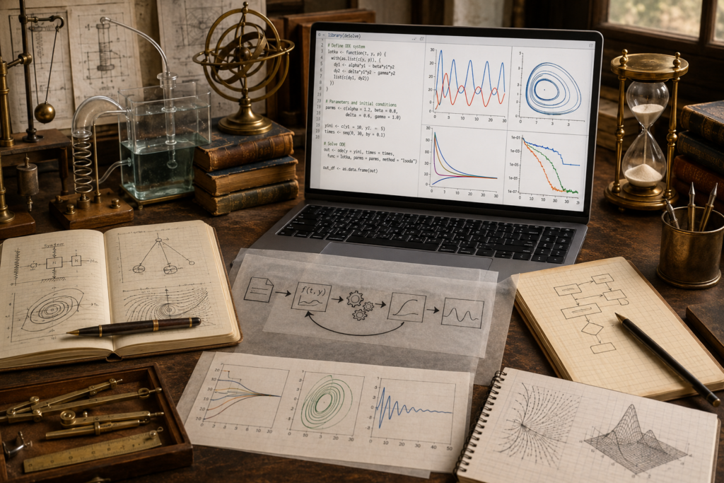

Calculus for Systems Modeling

Calculus for Systems Modeling examines how mathematical concepts of change, accumulation, rate, and continuous variation make it possible to analyze dynamic systems whose behavior unfolds across time. Within systems modeling, calculus provides a foundational framework for describing growth, decline, feedback, equilibrium, instability, optimization, and transition in domains such as ecology, economics, engineering, environmental science, physics, and sustainability.

This category explores the role of derivatives, integrals, differential equations, multivariable analysis, optimization, and numerical approximation in the study of complex systems. It considers how continuous processes can be formally represented, how interacting variables shape system behavior, and how mathematical structure can clarify the mechanisms through which systems evolve, stabilize, or break down. Particular attention is given to nonlinear dynamics, threshold effects, rates of change, and the analytical conditions under which intervention may amplify, dampen, or redirect systemic behavior.

The category also considers the relationship between formal mathematical reasoning and computational implementation. Calculus is not treated here as an abstract technical exercise alone, but as a practical and conceptual language for simulation, modeling, visualization, and reproducible analysis. Where appropriate, articles may connect classical calculus to Python-based workflows, numerical methods, and computational experiments that allow continuous systems to be studied in applied settings.

By linking mathematical analysis to systems thinking, this category situates calculus as an essential instrument for understanding temporal processes, causal structure, and the evolving behavior of complex systems.

Archival systems modeling workspace with bounded maps, contour fields, vector diagrams, landscape models, reservoirs, notebooks, translucent overlays, and drafting tools representing initial conditions, boundary conditions, and model scope.

Initial Conditions, Boundary Conditions, and Model Scope

Initial conditions, boundary conditions, and model scope define where a mathematical model begins, where it is allowed to operate, and what claims it can responsibly support. This article introduces these foundations for calculus-based systems modeling, including starting values, boundary rules, temporal horizons, spatial domains, parameter ranges, data domains, solver settings, sensitivity to starting assumptions, boundary effects, scope creep, and responsible interpretation. It shows why conditions and scope matter: differential equations require initial or boundary information to produce meaningful solutions, spatial models depend on edge behavior, and systems models can be misused when applied beyond their intended domain. In computational workflows, condition and scope audits support initial-condition tables, boundary-condition records, scope registries, SQL governance tables, Haskell typed records, calculator scripts, and generated reports. The article emphasizes documenting units, sources, uncertainty, domains, warnings, and claim boundaries for transparent, accountable model interpretation.
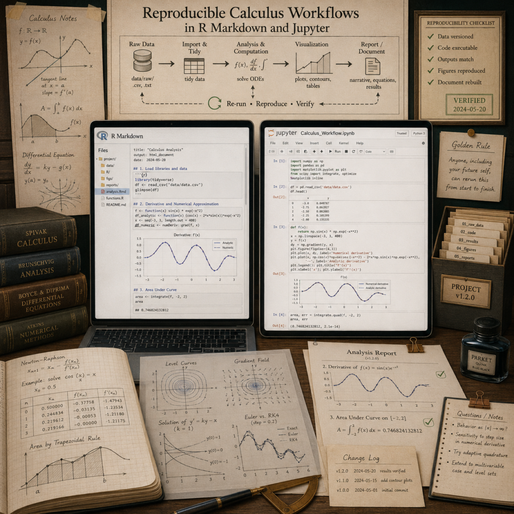
Scholarly computational workspace with R Markdown and Jupyter notebooks, calculus diagrams, code outputs, reports, versioned folders, checklists, notebooks, books, and drafting tools representing reproducible calculus workflows.

Reproducible Calculus Workflows in R Markdown, Jupyter, and Multi-Language Repositories

Reproducible calculus workflows make mathematical modeling transparent, inspectable, reusable, and easier to govern. This article introduces reproducible workflows for calculus-based systems modeling in R Markdown, Jupyter, and multi-language repositories, including executable documentation, parameter records, assumption logs, source data, generated outputs, clean-run checks, environment notes, CSV and JSON exports, SQL registries, Haskell typed records, calculator scripts, and governance queues. It shows why reproducibility matters: continuous models often depend on rates, accumulation, differential equations, numerical approximations, solver settings, calibration choices, sensitivity ranges, initial conditions, and assumptions about scale. In computational workflows, reproducibility audits support workflow artifact registers, run records, output metadata, diagnostic tables, Markdown reports, notebook placeholders, and repository smoke tests. The article emphasizes documenting equations, data status, parameters, units, commands, dependencies, outputs, diagnostics, warnings, and interpretation boundaries.

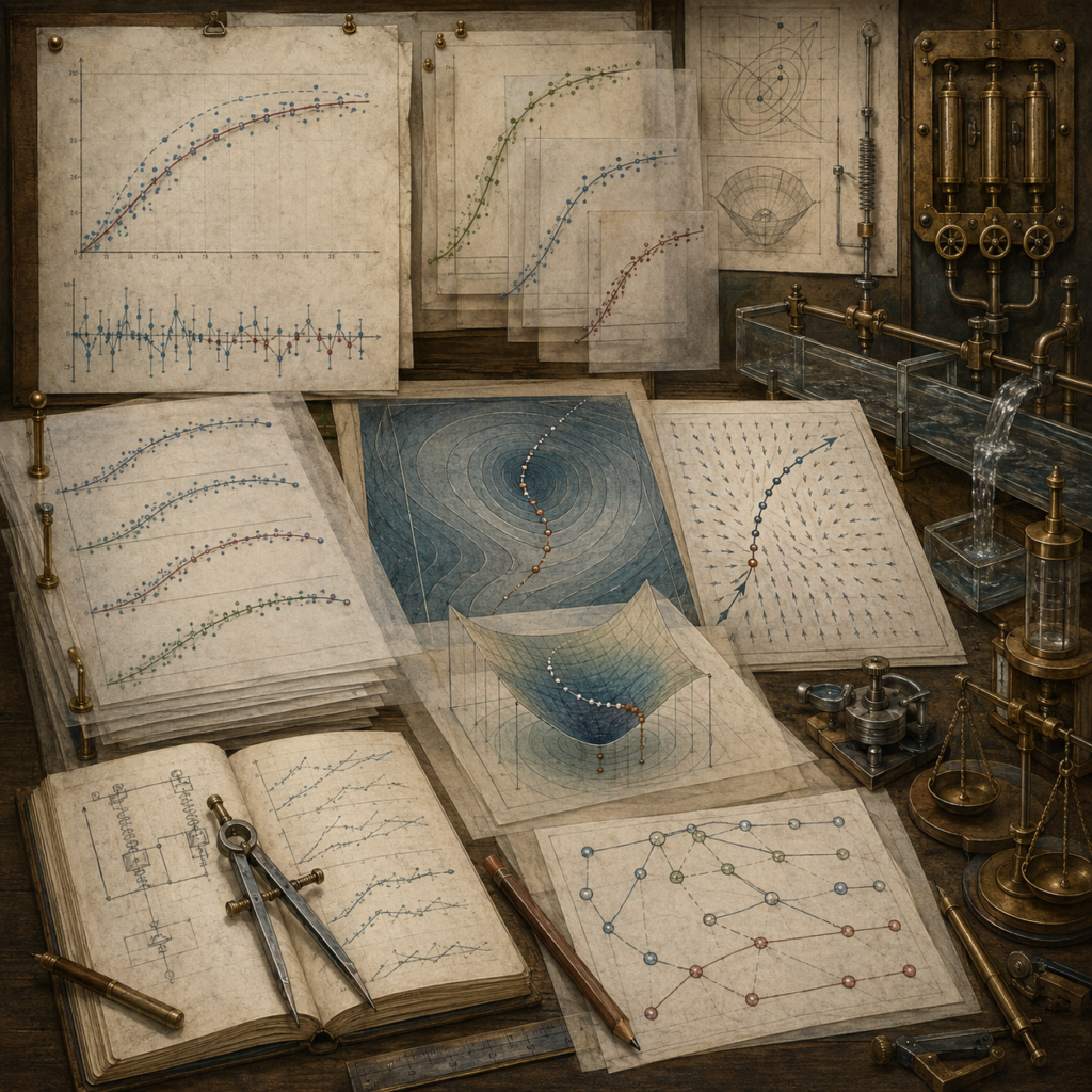
Archival systems modeling workspace with fitted curves, residual-like plots, contour surfaces, gradient paths, flow apparatuses, notebooks, balances, and drafting tools representing calculus-based model calibration.

Model Calibration Using Calculus-Based Methods

Model calibration using calculus-based methods connects mathematical structure with data by estimating parameters through residuals, loss functions, derivatives, gradients, Jacobians, Hessians, and optimization. This article introduces calibration for systems modeling, including least squares, objective functions, derivative-based optimization, parameter bounds, identifiability, overfitting, validation boundaries, calibration diagnostics, reproducible workflows, and responsible interpretation. It shows why calibration matters: population dynamics, epidemiological models, climate feedback, resource systems, infrastructure stress, economic adjustment, and spatial models often depend on uncertain rates, capacities, delays, elasticities, or feedback strengths. In computational workflows, calibration audits support synthetic teaching data, residual tables, candidate losses, best-fit parameter records, SQL governance registries, calculator scripts, and generated reports. The article emphasizes documenting calibration data, preprocessing, parameter definitions, units, bounds, starting values, loss functions, optimization methods, convergence status, residuals, uncertainty, validation limits, and interpretive warnings.

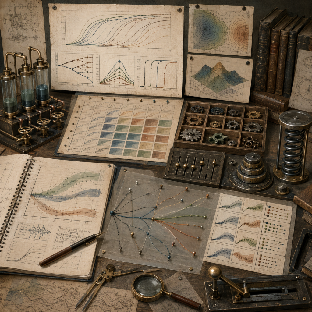
Vintage engineering and systems modeling workspace with parameter sweep charts, sensitivity curves, contour maps, surface plots, control sliders, gears, notebooks, and drafting tools representing sensitivity analysis.

Parameter Sweeps and Sensitivity Analysis

Parameter sweeps and sensitivity analysis reveal whether model conclusions are robust, fragile, or assumption-dependent. This article introduces sensitivity workflows for systems modeling, including one-at-a-time sweeps, grid sweeps, local sensitivity, global sensitivity, finite differences, elasticity-style measures, response surfaces, scenario envelopes, robustness review, fragility diagnosis, reproducible workflows, and responsible interpretation. It shows why sensitivity matters: population dynamics, epidemiological models, climate feedback, resource systems, infrastructure stress, economic adjustment, and coupled human-natural systems can change sharply when rates, capacities, delays, thresholds, elasticities, or initial conditions shift. In computational workflows, sensitivity audits support parameter tables, baseline records, sweep grids, local derivative estimates, robustness summaries, SQL governance registries, calculator scripts, and generated reports. The article emphasizes documenting parameter names, units, baselines, ranges, sources, sweep design, solver settings, output metrics, thresholds, interactions, and interpretive limits.

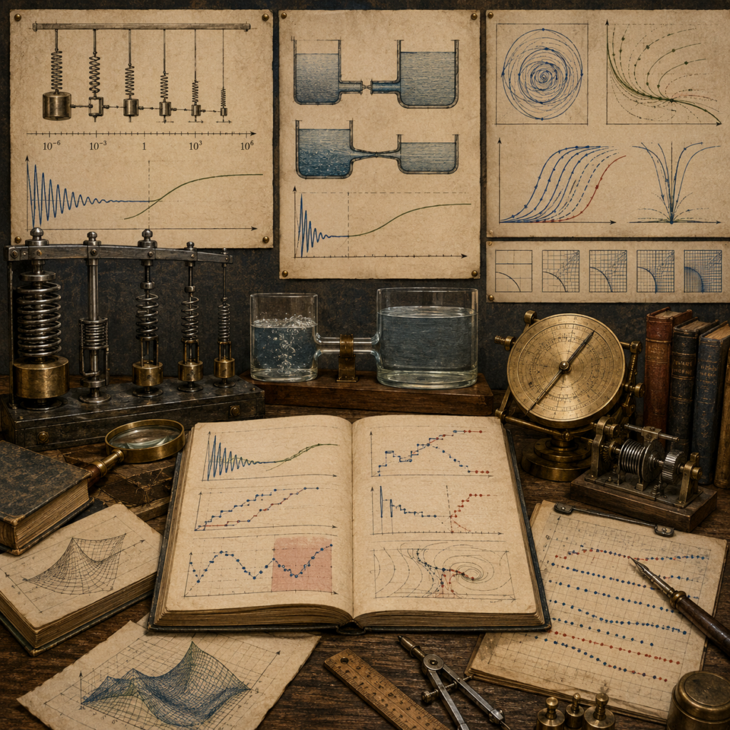
Vintage engineering and mathematical workspace with spring mechanisms, coupled reservoirs, rapidly decaying oscillations, slow response curves, phase diagrams, notebooks, gauges, and drafting tools representing stiff systems and computational difficulty.

Stiff Systems and Computational Difficulty in Numerical Modeling

Stiff systems and computational difficulty arise when dynamic models contain fast and slow processes that numerical solvers must handle together. This article introduces stiffness for systems modeling, including time-scale separation, explicit step-size limits, implicit methods, stability regions, adaptive solvers, stiffness warnings, Jacobian review, scaling, nondimensionalization, solver diagnostics, reproducible workflows, and responsible interpretation. It shows why stiffness matters: climate feedback, epidemiological transitions, infrastructure stress, chemical kinetics, ecological recovery, economic adjustment, and coupled human-natural systems may run slowly, fail, or produce misleading results when solver methods are poorly matched to model structure. In computational workflows, stiffness audits support explicit-implicit comparisons, amplification-factor checks, step-size difficulty tables, SQL governance registries, calculator scripts, and generated reports. The article emphasizes documenting solver method, time scales, tolerances, step histories, warnings, scaling choices, and interpretive limits so numerical difficulty becomes visible, auditable, and explained across modeling contexts.

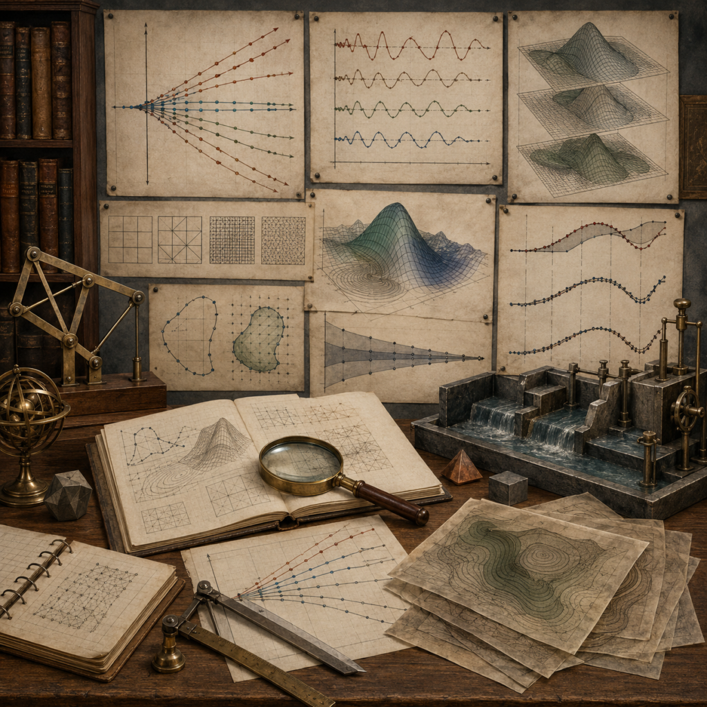
Vintage mathematical modeling workspace with stability diagrams, error trajectories, converging paths, mesh grids, surface plots, water-channel models, notebooks, brass instruments, and drafting tools.

Stability, Error, and Convergence in Numerical Modeling

Stability, error, and convergence in numerical modeling determine whether computed results can be trusted as computations. This article introduces numerical reliability for systems modeling, including local error, global error, truncation error, round-off error, consistency, numerical stability, convergence testing, step-size refinement, solver diagnostics, stiffness warnings, reproducible workflows, and responsible interpretation. It shows why numerical review matters: population dynamics, epidemiological models, climate feedback, resource systems, infrastructure stress, spatial dynamics, economic adjustment, and solver workflows can produce smooth-looking outputs that hide instability, under-resolution, accumulated error, or fragile assumptions. In computational workflows, convergence audits support RK4 benchmark comparisons, refinement tables, stability notes, diagnostic records, SQL governance registries, calculator scripts, and generated reports. The article emphasizes documenting solver method, step size, tolerances, benchmark values, residuals, warnings, constraint checks, and interpretive limits.

Scholarly computational workspace with two laptops showing continuous model visualizations, contour maps, surface plots, density fields, curve families, notebooks, brass tools, and drafting materials without labels or readable text.

Visualization of Continuous Models: Trajectories, Fields, Uncertainty, and Diagnostics

Visualization of continuous models turns equations, trajectories, fields, surfaces, uncertainty, and diagnostics into interpretable visual evidence. This article introduces visualization for systems modeling, including time trajectories, phase portraits, slope fields, vector fields, response surfaces, contour plots, uncertainty bands, sensitivity displays, diagnostic plots, reproducible graphics workflows, and responsible interpretation. It shows why visualization matters: population dynamics, epidemiological compartments, climate feedback, resource systems, infrastructure stress, spatial dynamics, economic adjustment, and numerical solver workflows often require visual inspection before results can be trusted. In computational workflows, visualization audits support trajectory tables, scenario comparisons, figure metadata, scale records, uncertainty notes, SQL governance registries, calculator scripts, and generated outputs. The article emphasizes documenting parameters, initial conditions, solver settings, units, axes, scales, transformations, grid resolution, color choices, smoothing, interpolation, uncertainty definitions, and interpretive limits.

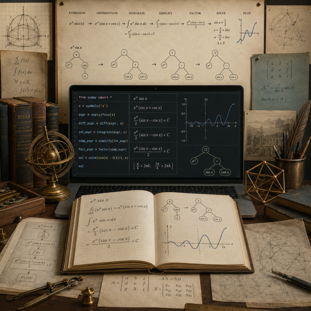
Editorial mathematical illustration of symbolic calculus and model inspection for systems modeling, showing exact equations, derivatives, integrals, limits, Jacobians, expression trees, simplification paths, assumption notes, notebooks, audit trails, and model review materials.

Symbolic Calculus and Model Inspection: Derivatives, Limits, Equilibria, and Structure

Symbolic calculus and model inspection use exact mathematical expressions to examine how a model is structured before numerical results are trusted. This article introduces symbolic calculus for systems modeling, including symbolic differentiation, integration, simplification, limits, Jacobians, Hessians, equilibrium analysis, boundary behavior, dimensional checks, expression governance, reproducible workflows, and responsible interpretation. It shows why symbolic inspection matters: population dynamics, epidemiological models, climate feedback, resource systems, economic adjustment, infrastructure models, and coupled dynamic systems often contain hidden assumptions, domain restrictions, singularities, equilibria, and parameter sensitivities that should be inspected before simulation. In computational workflows, symbolic model audits support expression records, derivative checks, equilibrium registries, limit analysis, Jacobian review, SQL assumption tables, calculator scripts, and generated reports. The article emphasizes documenting original expressions, transformed expressions, assumptions, domains, excluded values, parameter regimes, warnings, and interpretive limits.

Editorial mathematical illustration of ordinary differential equation solver workflows for systems modeling, showing state variables, rate equations, solver controls, time steps, tolerance settings, diagnostic charts, simulation outputs, notebooks, audit trails, and model review materials.

Ordinary Differential Equation Solver Workflows

Ordinary differential equation solver workflows turn dynamic equations into reproducible simulations. This article introduces ODE solver workflows for systems modeling, including initial value problems, state vectors, rate functions, fixed-step methods, adaptive solvers, tolerances, step-size controls, stiffness, diagnostics, validation, reproducibility, and model governance. It shows why solver workflows matter: population dynamics, epidemiological compartments, climate feedback, infrastructure stress, resource depletion, engineering systems, economic adjustment, and coupled feedback models often depend on solver configuration as much as equation structure. In computational workflows, ODE solver audits support RK4 benchmarks, step-size comparisons, tolerance records, stiffness warnings, solver-status logs, SQL assumption registries, calculator scripts, and generated outputs. The article emphasizes documenting equations, initial conditions, parameters, units, solver method, tolerances, event logic, output times, diagnostics, benchmark errors, software versions, and interpretive limits so numerical trajectories remain transparent, reproducible, and responsibly interpreted.

Scroll to Top