
Calculus for Systems Modeling

Calculus for Systems Modeling examines how mathematical concepts of change, accumulation, rate, and continuous variation make it possible to analyze dynamic systems whose behavior unfolds across time. Within systems modeling, calculus provides a foundational framework for describing growth, decline, feedback, equilibrium, instability, optimization, and transition in domains such as ecology, economics, engineering, environmental science, physics, and sustainability.

This category explores the role of derivatives, integrals, differential equations, multivariable analysis, optimization, and numerical approximation in the study of complex systems. It considers how continuous processes can be formally represented, how interacting variables shape system behavior, and how mathematical structure can clarify the mechanisms through which systems evolve, stabilize, or break down. Particular attention is given to nonlinear dynamics, threshold effects, rates of change, and the analytical conditions under which intervention may amplify, dampen, or redirect systemic behavior.

The category also considers the relationship between formal mathematical reasoning and computational implementation. Calculus is not treated here as an abstract technical exercise alone, but as a practical and conceptual language for simulation, modeling, visualization, and reproducible analysis. Where appropriate, articles may connect classical calculus to Python-based workflows, numerical methods, and computational experiments that allow continuous systems to be studied in applied settings.

By linking mathematical analysis to systems thinking, this category situates calculus as an essential instrument for understanding temporal processes, causal structure, and the evolving behavior of complex systems.

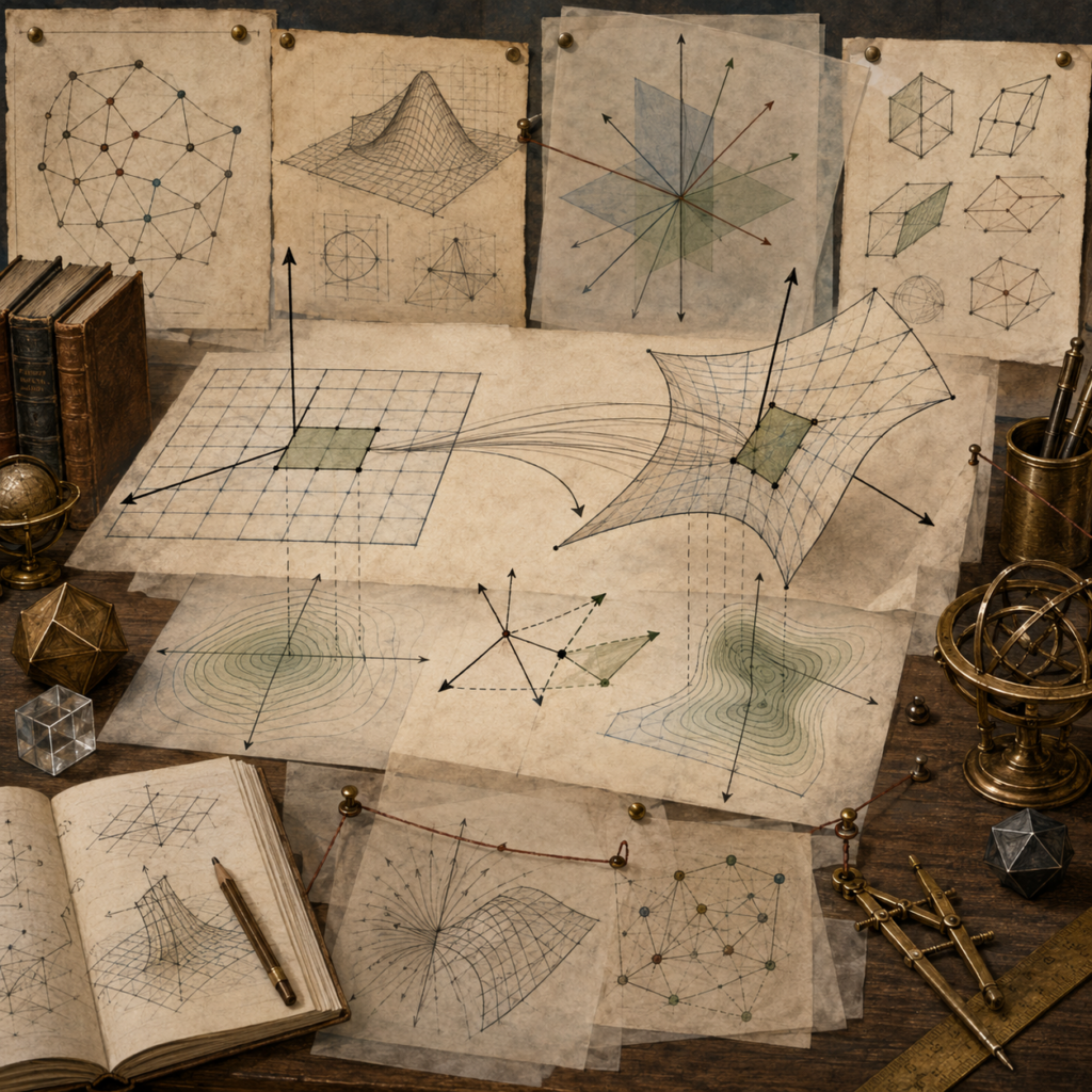
Editorial mathematical illustration of vectors, fields, and continuous space in systems modeling, showing vector arrows, scalar surfaces, spatial grids, flow lines, contour maps, coordinate axes, notebooks, and computational modeling materials.

Vectors, Fields, and Continuous Space

Vectors, fields, and continuous space give systems modeling a language for direction, magnitude, location, interaction, and spatial variation. This article explains vectors, coordinate components, vector magnitude, dot products, scalar fields, vector fields, continuous domains, field lines, contours, streamlines, discrete data, gridded approximation, interpolation, units, field visualization, and smoothness assumptions. It shows why fields are not merely visual maps: they are mathematical claims that assign quantities or directions across a defined domain. In computational workflows, vector and field audits support scalar-field diagnostics, vector-magnitude checks, domain review, grid-resolution comparison, unit documentation, synthetic spatial examples, and governance of field-based modeling assumptions. The article emphasizes that field claims should state the domain, units, coordinate convention, data source, resolution, interpolation method, smoothness assumption, and interpretive limits before using gradients, flux, circulation, or conservation reasoning.
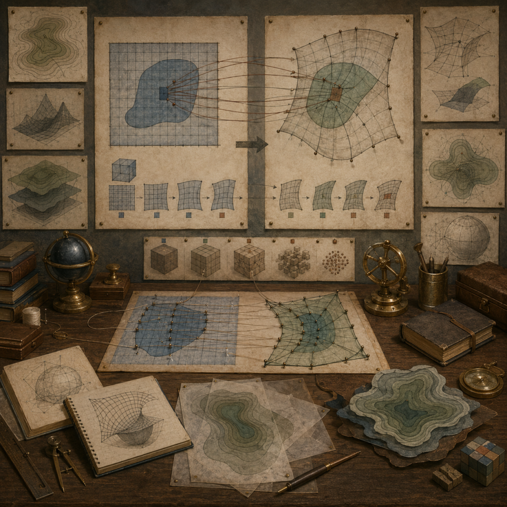

Editorial mathematical illustration of change of variables in multidimensional systems, showing transformed coordinate grids, mapped regions, Jacobian scaling, density fields, area and volume elements, notebooks, diagrams, and computational modeling materials.

Change of Variables in Multidimensional Systems

Change of variables in multidimensional systems explains how regions, coordinates, densities, and accumulated quantities transform when a model is rewritten in another coordinate system. This article explains transformation maps, mapped domains, Jacobian matrices, Jacobian determinants, area and volume scaling, polar coordinates, cylindrical coordinates, spherical coordinates, density conservation, probability transformations, state-space transformations, orientation, singularity, invertibility, numerical reparameterization, and computational diagnostics. It shows why changing variables is not merely changing notation: the transformation changes how local area, volume, density, and accumulated totals must be measured. In computational workflows, change-of-variables audits support Jacobian checks, transformed-integral comparisons, coordinate-system diagnostics, density-conservation review, region-mapping validation, and governance of transformed models. The article emphasizes documenting the map, domain, determinant, scaling factor, units, invertibility, singular regions, and original-system interpretation.

Editorial mathematical illustration of multiple integrals and spatial accumulation in systems modeling, showing layered spatial regions, density fields, grid cells, contour surfaces, volumetric accumulation, notebooks, maps, and computational modeling materials.

Multiple Integrals and Spatial Accumulation

Multiple integrals extend accumulation from one-dimensional change to regions, surfaces, volumes, fields, and spatially distributed systems. This article explains how double integrals, triple integrals, density functions, regions, boundaries, domains, iterated integrals, coordinate systems, area and volume elements, spatial averages, weighted aggregation, gridded data, numerical integration, masks, resolution, and units shape systems modeling. It shows why multiple integrals are not merely larger definite integrals: they turn local quantities into totals over spatial domains, and those totals depend on what is being accumulated, where boundaries are drawn, how density is measured, and how geometry is represented. In computational workflows, multiple integrals support spatial accumulation audits, exposure-burden calculations, gridded approximation, population weighting, region-mask diagnostics, and governance of spatial aggregation claims. The article emphasizes documenting density, region, measure, resolution, boundary, weighting, and uncertainty.

Editorial mathematical illustration of constrained optimization and Lagrange multipliers in systems modeling, showing feasible regions, contour surfaces, constraint curves, tangent conditions, optimization worktables, notebooks, and computational modeling materials.

Constrained Optimization and Lagrange Multipliers

Constrained optimization asks how a system can improve, minimize loss, or balance competing objectives when movement is limited by feasibility conditions. This article explains how objectives, equality constraints, inequality constraints, feasible regions, boundary conditions, Lagrange multipliers, gradient balance, tangency, shadow values, active constraints, constraint residuals, second-order feasible-direction checks, units, scaling, and local validity shape systems modeling. It shows why constrained optimization is not simply optimization with an extra equation: it changes the interpretation from best unconstrained movement to best feasible movement. In computational workflows, constrained optimization supports feasibility audits, stationarity checks, multiplier diagnostics, active-boundary review, resource-allocation analysis, policy tradeoff interpretation, and governance of formal decision support. The article emphasizes that optimization claims should state the objective, constraints, units, scaling, active status, residuals, multiplier meaning, and local-validity limits.

Editorial mathematical illustration of Hessians, curvature, and local structure in systems modeling, showing curved response surfaces, second-derivative matrices, saddle shapes, contour maps, local neighborhoods, notebooks, and computational modeling materials.

Hessians, Curvature, and Local Structure: Second-Order Calculus for Systems Modeling

Hessians extend calculus from first-order sensitivity to second-order local structure, showing how curvature, interaction, acceleration, and changing marginal response shape multivariable systems. This article explains how Hessian matrices, second partial derivatives, cross partials, quadratic forms, convexity, concavity, saddle points, eigenvalue signs, conditioning, critical points, second-order approximation, reference states, and local validity support systems modeling. It shows why a Hessian is not merely a matrix of second derivatives: it is a local curvature map that depends on where it is evaluated, how variables are scaled, whether feasible directions are constrained, and whether smoothness assumptions hold. In computational workflows, Hessians support curvature audits, optimization diagnostics, approximation-error comparison, saddle detection, cross-partial review, parameter identifiability checks, and governance of nonlinear sensitivity claims. The article emphasizes careful documentation of reference points, units, derivative method, curvature classification, and local-validity limits.

Editorial mathematical illustration of Jacobians and multivariable transformation in systems modeling, showing input grids transformed into output grids, local linear maps, matrix structures, coordinate transformations, notebooks, contour maps, and computational modeling materials.

Jacobians and Multivariable Transformation: How Calculus Maps Local System Change

Jacobians organize how multivariable systems transform local movement, sensitivity, area, volume, and structure across dimensions. This article explains how Jacobian matrices, vector-valued functions, local linear maps, input-output sensitivity matrices, coordinate transformations, determinant scaling, singularity, conditioning, dynamic-system stability, reference states, and local validity shape systems modeling. It shows why a Jacobian is not merely a table of partial derivatives: it is a local transformation rule that depends on where it is evaluated, how inputs and outputs are defined, what units and scaling are used, and whether perturbations are feasible. In computational workflows, Jacobians support sensitivity auditing, solver diagnostics, coordinate-change checks, determinant review, stability analysis, approximation-error testing, and transformation governance. The article emphasizes that Jacobian claims should state the reference point, matrix orientation, units, derivative method, determinant or conditioning warnings, and local-validity region.

Editorial mathematical illustration of directional derivatives and gradients in systems modeling, showing contour maps, gradient arrows, local direction vectors, multivariable surfaces, tangent-plane sketches, notebooks, and computational modeling materials.

Directional Derivatives and Gradients: How Calculus Tracks Local Change Across System Pathways

Directional derivatives and gradients extend local sensitivity from coordinate-by-coordinate change to movement in any chosen direction through multivariable input space. This article explains how direction vectors, unit normalization, gradients, gradient norms, dot products, steepest increase, steepest decrease, contour geometry, feasible directions, scaling, units, reference states, and local validity shape systems modeling. It shows why directional derivatives are not merely formulas: they depend on where the gradient is evaluated, how the direction is defined, whether units have been normalized, whether movement is feasible, and whether the approximation remains local. In computational workflows, directional derivatives support scenario-path analysis, gradient diagnostics, feasible-direction checks, approximation-error review, and sensitivity interpretation. The article emphasizes that gradient claims should state the reference point, direction vector, normalization rule, units, constraints, and local-validity region before supporting responsible interpretation across complex systems, especially in constrained, nonlinear, and dynamic settings.

Editorial mathematical illustration of total differentials and local approximation in higher dimensions, showing tangent planes, multivariable surfaces, gradient arrows, small perturbation vectors, local neighborhoods, notebooks, contour maps, and computational modeling materials.

Total Differentials and Local Approximation: How Calculus Estimates Multivariable System Change

Total differentials extend partial derivatives into a disciplined estimate of how a multivariable system changes when several inputs shift at once. This article explains how partial derivatives, displacement vectors, tangent planes, gradient notation, local linear approximation, error propagation, feasible movement, constraints, reference states, and local validity shape systems modeling. It shows why total differentials are not global forecasts: they are first-order approximations tied to a specific point, small perturbations, smoothness assumptions, and meaningful movement through input space. In computational workflows, total differentials support uncertainty propagation, sensitivity accounting, scenario adjustment, approximation-error checks, and feasibility review. The article emphasizes that differential claims should state the reference point, displacement vector, partial derivatives, constraints, and local-validity region before supporting responsible interpretation across complex systems, especially when small perturbations are used to explain uncertainty, policy adjustment, or near-baseline change in dynamic, constrained, nonlinear models.

Editorial mathematical illustration of partial derivatives and interaction effects in systems modeling, showing multivariable surfaces, tangent slices, contour maps, interaction grids, derivative notes, notebooks, and computational modeling materials.

Partial Derivatives and Interaction Effects: How Calculus Measures Local System Sensitivity

Partial derivatives measure how a multivariable system changes when one input changes while other inputs are held fixed. This article explains how coordinate slices, fixed-variable assumptions, local sensitivity, marginal response, interaction terms, cross-partial derivatives, feasible regions, constraints, contour interpretation, reference states, and local validity shape systems modeling. It shows why partial derivatives are not context-free numbers: they depend on where they are evaluated, which variables are held constant, whether inputs can vary independently, and whether interactions change sensitivity across the input space. In modeling workflows, partial derivatives support sensitivity grids, interaction diagnostics, feasible-change checks, cross-partial review, and local approximation. The article emphasizes that derivative claims should state the reference point, fixed variables, units, constraints, and interaction structure before supporting responsible interpretation across complex systems, where local rates can mislead when used as global causal or policy claims too broadly.

Scroll to Top