
Author name: Tariq Ahmad

Editorial mathematical illustration of gradient, divergence, and curl in systems modeling, showing scalar fields, vector fields, directional arrows, spreading flow, rotational structure, spatial grids, notebooks, and computational modeling materials.

Gradient, Divergence, and Curl

Gradient, divergence, and curl are local vector-calculus operators that reveal how fields change, spread, converge, rotate, and organize motion through continuous space. This article explains scalar fields, vector fields, the del operator, gradient, divergence, curl, gradient magnitude, source-sink behavior, rotational tendency, finite-difference approximation, grid spacing, coordinate systems, units, boundary handling, smoothing, flux, circulation, and responsible interpretation. It shows why these operators are not interchangeable: gradient maps scalar fields to directional change, divergence maps vector fields to local spreading or convergence, and curl maps vector fields to local rotation. In computational workflows, field-operator audits support gradient diagnostics, divergence checks, curl summaries, grid-resolution review, SQL assumption registries, calculator scripts, and governance of spatial-field claims. The article emphasizes documenting field meaning, units, coordinates, derivative method, smoothing, boundary rules, and interpretive limits.


Editorial mathematical illustration of surface integrals and distributed accumulation in systems modeling, showing curved surfaces, flux arrows, density fields, surface patches, normal vectors, boundaries, spatial grids, notebooks, and computational modeling materials.

Surface Integrals and Distributed Accumulation

Surface integrals measure accumulation across a surface rather than along a path or throughout a volume. This article explains scalar surface integrals, vector surface integrals, flux, oriented surfaces, normal vectors, surface parameterization, surface-area elements, tangent vectors, cross products, mesh patches, boundary surfaces, distributed accumulation, computational approximation, and responsible interpretation. It shows why surface integrals are not merely double integrals on curved objects: they answer interface-based questions about pressure, heat, exposure, load, radiation, airflow, water flow, emissions, and boundary crossing. In computational workflows, surface-integral audits support patch sampling, surface-area approximation, scalar accumulation, vector flux diagnostics, normal-orientation checks, mesh-resolution review, SQL assumption registries, calculator scripts, and governance of boundary-based claims. The article emphasizes documenting the surface, field, orientation, area element, units, boundary meaning, interpolation, mesh resolution, and interpretive limits.

Editorial mathematical illustration of line integrals and paths through space in systems modeling, showing curved trajectories, scalar field accumulation, vector field arrows, work, circulation, spatial grids, notebooks, and computational modeling materials.

Line Integrals and Paths Through Space

Line integrals measure accumulation along a path rather than across an area or volume. This article explains scalar line integrals, vector line integrals, parameterized curves, arc-length elements, field-path interaction, work, circulation, path dependence, conservative fields, state-space line integrals, computational approximation, segment sampling, scalar accumulation, vector dot products, alignment diagnostics, and responsible interpretation. It shows why line integrals are not merely integrals drawn over curves: they answer path-based questions about exposure, work, cost, resistance, flow support, circulation, and route history. In computational workflows, line-integral audits support path sampling, path-length approximation, scalar-field accumulation, vector-field interaction, alignment review, SQL assumption registries, calculator scripts, and governance of path-based claims. The article emphasizes documenting the path, field, direction, units, parameterization, interpolation, sampling resolution, accumulated quantity, and interpretive limits.

Editorial mathematical illustration of vector-valued functions and motion in systems modeling, showing parameterized trajectories, position vectors, velocity arrows, acceleration vectors, curved paths, spatial grids, notebooks, and computational modeling materials.

Vector-Valued Functions and Motion

Vector-valued functions describe motion by assigning a position vector to each value of time or another parameter. This article explains parameterized curves, component functions, position vectors, velocity, acceleration, speed, direction, unit tangent vectors, arc length, distance traveled, displacement, path efficiency, curvature, state-space trajectories, computational sampling, finite-difference estimates, and motion diagnostics. It shows why vector-valued functions are not merely several scalar formulas: they describe coordinated movement through space or state space. In computational workflows, trajectory audits support position sampling, speed calculation, arc-length approximation, displacement comparison, path-efficiency checks, velocity estimation, time-step review, state-space scaling, SQL assumption registries, and governance of motion claims. The article emphasizes documenting parameter meaning, component units, coordinate systems, time interval, sampling resolution, smoothing assumptions, scaling choices, and interpretive limits before drawing conclusions about trajectory behavior.

Editorial mathematical illustration of vectors, fields, and continuous space in systems modeling, showing vector arrows, scalar surfaces, spatial grids, flow lines, contour maps, coordinate axes, notebooks, and computational modeling materials.

Vectors, Fields, and Continuous Space

Vectors, fields, and continuous space give systems modeling a language for direction, magnitude, location, interaction, and spatial variation. This article explains vectors, coordinate components, vector magnitude, dot products, scalar fields, vector fields, continuous domains, field lines, contours, streamlines, discrete data, gridded approximation, interpolation, units, field visualization, and smoothness assumptions. It shows why fields are not merely visual maps: they are mathematical claims that assign quantities or directions across a defined domain. In computational workflows, vector and field audits support scalar-field diagnostics, vector-magnitude checks, domain review, grid-resolution comparison, unit documentation, synthetic spatial examples, and governance of field-based modeling assumptions. The article emphasizes that field claims should state the domain, units, coordinate convention, data source, resolution, interpolation method, smoothness assumption, and interpretive limits before using gradients, flux, circulation, or conservation reasoning.

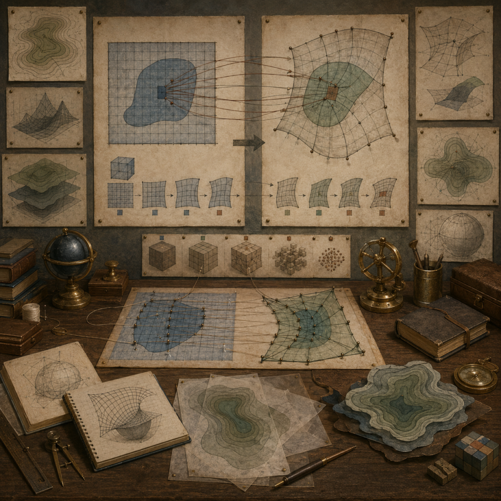
Editorial mathematical illustration of change of variables in multidimensional systems, showing transformed coordinate grids, mapped regions, Jacobian scaling, density fields, area and volume elements, notebooks, diagrams, and computational modeling materials.

Change of Variables in Multidimensional Systems

Change of variables in multidimensional systems explains how regions, coordinates, densities, and accumulated quantities transform when a model is rewritten in another coordinate system. This article explains transformation maps, mapped domains, Jacobian matrices, Jacobian determinants, area and volume scaling, polar coordinates, cylindrical coordinates, spherical coordinates, density conservation, probability transformations, state-space transformations, orientation, singularity, invertibility, numerical reparameterization, and computational diagnostics. It shows why changing variables is not merely changing notation: the transformation changes how local area, volume, density, and accumulated totals must be measured. In computational workflows, change-of-variables audits support Jacobian checks, transformed-integral comparisons, coordinate-system diagnostics, density-conservation review, region-mapping validation, and governance of transformed models. The article emphasizes documenting the map, domain, determinant, scaling factor, units, invertibility, singular regions, and original-system interpretation.

Editorial mathematical illustration of multiple integrals and spatial accumulation in systems modeling, showing layered spatial regions, density fields, grid cells, contour surfaces, volumetric accumulation, notebooks, maps, and computational modeling materials.

Multiple Integrals and Spatial Accumulation

Multiple integrals extend accumulation from one-dimensional change to regions, surfaces, volumes, fields, and spatially distributed systems. This article explains how double integrals, triple integrals, density functions, regions, boundaries, domains, iterated integrals, coordinate systems, area and volume elements, spatial averages, weighted aggregation, gridded data, numerical integration, masks, resolution, and units shape systems modeling. It shows why multiple integrals are not merely larger definite integrals: they turn local quantities into totals over spatial domains, and those totals depend on what is being accumulated, where boundaries are drawn, how density is measured, and how geometry is represented. In computational workflows, multiple integrals support spatial accumulation audits, exposure-burden calculations, gridded approximation, population weighting, region-mask diagnostics, and governance of spatial aggregation claims. The article emphasizes documenting density, region, measure, resolution, boundary, weighting, and uncertainty.

Editorial mathematical illustration of constrained optimization and Lagrange multipliers in systems modeling, showing feasible regions, contour surfaces, constraint curves, tangent conditions, optimization worktables, notebooks, and computational modeling materials.

Constrained Optimization and Lagrange Multipliers

Constrained optimization asks how a system can improve, minimize loss, or balance competing objectives when movement is limited by feasibility conditions. This article explains how objectives, equality constraints, inequality constraints, feasible regions, boundary conditions, Lagrange multipliers, gradient balance, tangency, shadow values, active constraints, constraint residuals, second-order feasible-direction checks, units, scaling, and local validity shape systems modeling. It shows why constrained optimization is not simply optimization with an extra equation: it changes the interpretation from best unconstrained movement to best feasible movement. In computational workflows, constrained optimization supports feasibility audits, stationarity checks, multiplier diagnostics, active-boundary review, resource-allocation analysis, policy tradeoff interpretation, and governance of formal decision support. The article emphasizes that optimization claims should state the objective, constraints, units, scaling, active status, residuals, multiplier meaning, and local-validity limits.

Editorial mathematical illustration of Hessians, curvature, and local structure in systems modeling, showing curved response surfaces, second-derivative matrices, saddle shapes, contour maps, local neighborhoods, notebooks, and computational modeling materials.

Hessians, Curvature, and Local Structure: Second-Order Calculus for Systems Modeling

Hessians extend calculus from first-order sensitivity to second-order local structure, showing how curvature, interaction, acceleration, and changing marginal response shape multivariable systems. This article explains how Hessian matrices, second partial derivatives, cross partials, quadratic forms, convexity, concavity, saddle points, eigenvalue signs, conditioning, critical points, second-order approximation, reference states, and local validity support systems modeling. It shows why a Hessian is not merely a matrix of second derivatives: it is a local curvature map that depends on where it is evaluated, how variables are scaled, whether feasible directions are constrained, and whether smoothness assumptions hold. In computational workflows, Hessians support curvature audits, optimization diagnostics, approximation-error comparison, saddle detection, cross-partial review, parameter identifiability checks, and governance of nonlinear sensitivity claims. The article emphasizes careful documentation of reference points, units, derivative method, curvature classification, and local-validity limits.

Scroll to Top