
Last Updated May 28, 2026
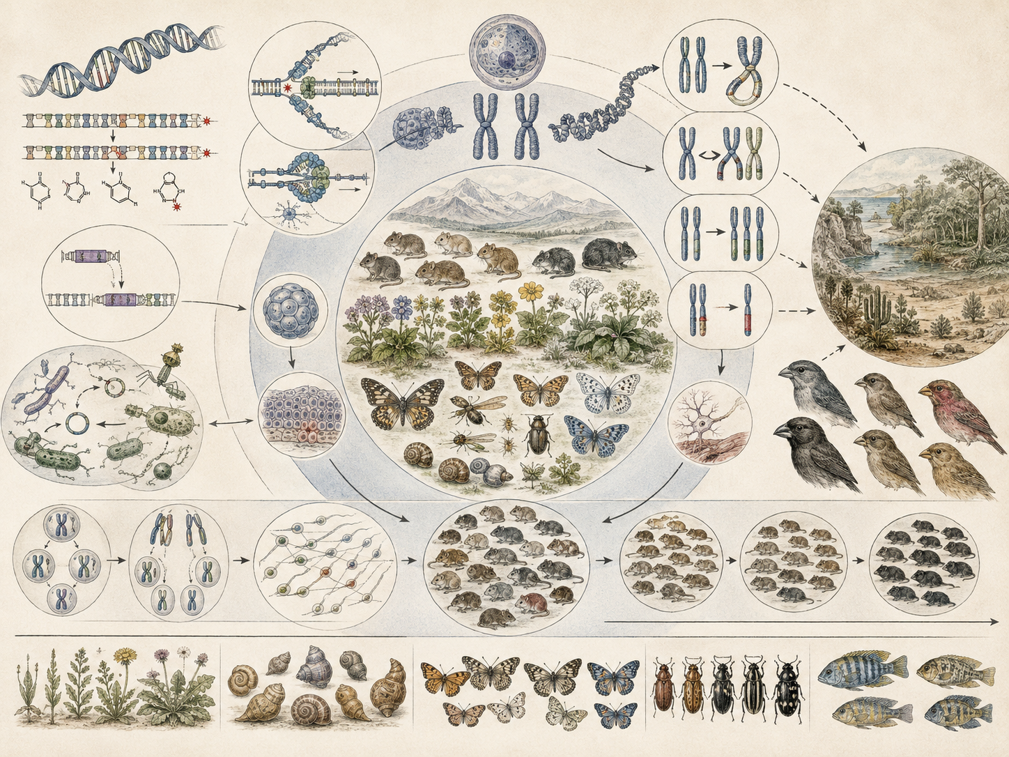
Mutation, variation, and the sources of novelty examine how living systems generate difference, preserve inherited diversity, redistribute biological possibility, and produce the raw material from which development, adaptation, disease, ecological resilience, and evolutionary change become possible. Novelty is one of biology’s most important problems because life persists not only through continuity, but also through the production of new forms, new combinations, new regulatory states, and new functional capacities under changing conditions. Mutation is one source of sequence change. Variation is the broader field of inherited, genomic, developmental, and phenotypic difference. Novelty is the emergence of traits, combinations, structures, regulatory patterns, or functions that become biologically consequential across cells, organisms, populations, ecosystems, or lineages.
This article develops Mutation, Variation, and the Sources of Novelty as a foundational article within the Biology knowledge series. It treats mutation not as a simple synonym for evolution, but as one molecular source of difference among many. It treats variation not as background noise, but as the distributed field of biological possibility on which selection, drift, recombination, repair, development, and ecology act. It treats novelty not as a mysterious sudden invention, but as a historically conditioned outcome of sequence change, standing variation, recombination, structural rearrangement, regulatory repatterning, developmental modularity, and ecological opportunity.
Main Library
Publications
Article Map
Biology
Related Topic
Chemistry
Related Topic
Earth Science
Related Topic
Environmental Science
The article develops mutation, variation, and biological novelty across point mutation, DNA repair, genome maintenance, mutation spectra, standing genetic variation, recombination, structural variation, genomic rearrangement, gene duplication, regulatory novelty, cryptic variation, mutation supply, nucleotide diversity, mutation-selection balance, mutation-selection-drift dynamics, microbial evolution, pathogen resistance, cancer genomics, conservation genetics, plant breeding, disease ecology, and computational variation analysis.
The article is written for geneticists, evolutionary biologists, developmental biologists, microbiologists, conservation biologists, plant scientists, medical and environmental-health readers, cancer-genomics readers, disease ecologists, bioinformaticians, computational biology readers, biodiversity experts, agroecologists, restoration practitioners, and systems biologists who need a rigorous account of how biological difference is generated, maintained, filtered, interpreted, and translated into future possibility.
The article also extends mutation and variation into quantitative and computational biology through allele-frequency reasoning, Hardy-Weinberg expectations, mutation-count models, Poisson mutation supply, sequence divergence, Jukes-Cantor distance, nucleotide diversity, site-frequency spectra, mutation spectra, mutation-selection balance, mutation-selection-drift simulations, structural-variation priority scoring, R workflows, Python workflows, SQL provenance structures, and a linked full-stack GitHub repository containing Python, R, Julia, Fortran, Rust, Go, C, C++, SQL, notebooks, data files, validation notes, and reproducibility documentation.
What mutation, variation, and novelty are
Mutation refers to a change in the DNA sequence of an organism, cell lineage, or genetic system. Variation refers more broadly to genetic, genomic, developmental, physiological, and phenotypic differences among individuals, populations, lineages, or communities. Novelty refers to the emergence of new traits, new combinations, new structures, new regulatory states, or new functional possibilities that were not previously present in the same form. These concepts are related, but they are not identical. Mutation is one source of variation. Variation is one condition that makes novelty possible. Novelty emerges only when differences become biologically consequential across development, function, ecology, disease, or evolution.
This distinction matters because biology does not treat all difference in the same way. A mutation may occur without producing an important phenotypic effect. A population may carry substantial standing variation without immediately expressing evolutionary novelty. A novel trait may arise not from a single new mutation, but from new combinations of existing variants, altered regulation, structural rearrangement, gene duplication, hybridization, or developmental reorganization. Biology is therefore strongest when it distinguishes sequence change, inherited diversity, expressed difference, and functional novelty as connected but separable levels of explanation.
Mutation and variation also clarify one of life’s deepest tensions: living systems require continuity, but they also remain open to change. Heredity depends on stable transmission. Development depends on regulated reproducibility. Physiology depends on organized function. Yet adaptation, diversification, resistance, disease evolution, and new forms of life all require difference. Mutation and variation make biological history possible because they allow life to remain continuous without remaining fixed.
In that sense, mutation, variation, and novelty belong to the foundations of modern biology. They explain how living systems can preserve lineage identity while still generating new possibility. Life is not merely the repetition of inherited forms. It is continuity under conditions of difference, constraint, repair, recombination, selection, and ecological opportunity.
From mutation to novelty: a scale-spanning framework
Mutation becomes scientifically meaningful only when it is followed across scales. A nucleotide change may alter a codon, a regulatory motif, a splice site, a chromatin context, a structural interval, or nothing detectable at all. A variant may remain rare, drift to loss, rise under selection, persist in heterozygotes, become part of a haplotype, or interact with other variants in ways that change phenotype. A population may carry variation that is invisible under ordinary conditions but decisive under drought, infection, heat stress, chemical exposure, altered diet, or new ecological interaction.
The strongest account of biological novelty therefore moves from molecular event to population process, from population process to developmental expression, from developmental expression to organismal function, and from organismal function to ecological and evolutionary consequence. This avoids two common simplifications: treating every mutation as if it immediately produces adaptation, and treating novelty as if it appears without material or historical sources. Novelty usually emerges from an interaction among mutation, recombination, standing variation, regulation, development, ecological opportunity, and selective or stochastic filtering.
This scale-spanning view is especially important for modern biology because data now arrive at many levels simultaneously. Sequencing reveals variants. Functional genomics reveals regulatory effects. Developmental biology reveals whether those effects can produce viable form. Population genetics reveals whether variants spread, persist, or disappear. Ecology reveals whether the expressed difference matters in the world. Mutation and variation are therefore not merely topics within genetics; they are connecting concepts that help integrate molecular biology, development, ecology, evolution, medicine, conservation, agriculture, and computational biology.
Mutation as sequence change
Mutation is classically understood as a change in DNA sequence. This basic definition remains foundational because it identifies mutation as one of the principal molecular sources of new hereditary difference. Yet mutation is not biologically uniform. Some mutations are single-nucleotide substitutions. Others involve insertions, deletions, inversions, duplications, translocations, copy-number changes, mobile-element insertions, repeat expansions, or larger chromosomal rearrangements. Some occur in coding regions. Others occur in regulatory regions, introns, enhancers, promoters, noncoding RNA genes, structural genomic regions, or repetitive sequence.
Mutation is therefore best understood as a source of potential difference rather than as automatic innovation. It creates possibilities. Whether those possibilities remain neutral, become deleterious, or support adaptation depends on genomic location, inheritance, gene regulation, repair, population size, developmental viability, ecological condition, genetic background, and selection. A useful scientist-facing treatment of mutation must therefore include not just the existence of sequence change, but also mutation rate, mutation spectrum, repair dynamics, genomic context, inheritance mode, and the probability that a new event survives stochastic loss long enough to matter.
This also means mutation cannot be treated as a single uniform clock. Different lineages, loci, genome compartments, environmental exposures, replication systems, and repair pathways produce different mutational regimes. Mitochondrial genomes, nuclear genomes, microbial genomes, viral genomes, cancer cell lineages, germline cells, somatic tissues, and environmental DNA systems can all show different mutational dynamics. Mutation is foundational, but its consequences are filtered through genome maintenance, recombination, developmental viability, population structure, and ecological history.
A mutation is therefore a molecular event whose biological meaning depends on the system in which it occurs. A synonymous substitution may be largely neutral in one context but influence translation or regulation in another. A regulatory mutation may have no visible effect under ordinary conditions but matter under stress. A structural variant may be harmless in one genetic background and highly consequential in another. Mutation matters because it produces difference, but biology must still ask what that difference does.
This interpretive discipline is essential because mutation language often becomes misleading when detached from mechanism. Calling a variant “new,” “rare,” “deleterious,” “beneficial,” or “adaptive” requires evidence about inheritance, expression, population frequency, functional effect, and environment. A scientist-facing account of mutation therefore needs careful vocabulary: sequence change is not automatically function change, and function change is not automatically evolutionary success.
DNA repair, genome maintenance, and mutational processes
Mutation must be understood in relation to DNA repair and genome maintenance. Cells are not passive containers of genetic material. DNA is continually exposed to replication errors, chemical damage, radiation, reactive oxygen species, mobile elements, recombination errors, and structural stress. Living systems therefore invest heavily in repair and surveillance mechanisms that reduce, correct, tolerate, or route different kinds of damage. Mutation is not only a result of damage; it is also a result of how damage is prevented, repaired, misrepaired, or passed through replication.
This matters because mutation rates are shaped by biological systems that maintain genome integrity. Polymerase fidelity, proofreading, mismatch repair, base excision repair, nucleotide excision repair, double-strand break repair, homologous recombination, nonhomologous end joining, translesion synthesis, and checkpoint systems all influence the frequency and spectrum of mutations that persist. When repair fails or becomes compromised, mutation burden can increase dramatically, with consequences for cancer, aging, inherited disease, microbial evolution, environmental mutagenesis, and pathogen adaptation.
Genome maintenance also introduces a paradox. Life requires continuity, but evolution requires difference. Too much mutation can destroy function, reduce viability, or produce disease. Too little variation can reduce adaptive potential and limit future response. Mutation therefore belongs to a balance between stability and change. Biology preserves the fidelity of inheritance while never eliminating the possibility of novelty entirely.
This balance is not the same in every lineage or tissue. Germline mutation, somatic mutation, cancer mutation, microbial mutation, viral mutation, organellar mutation, and environmentally induced damage all occupy different biological contexts. Repair systems therefore do more than prevent error; they shape the landscape of possible future variation by determining which changes are corrected, tolerated, transmitted, or amplified.
This balance is especially important in high-stakes biological systems. In germline cells, mutation can shape future generations. In somatic tissues, mutation can contribute to cancer or age-related decline. In microbes and viruses, mutation can support rapid adaptation, resistance, or host shifts. In conservation biology, mutation may slowly replenish variation, but often too slowly to compensate for rapid population collapse. Mutation is therefore always both molecular and historical.
Variation as a biological field of difference
Variation is broader than mutation because it includes all the inherited and genomic differences distributed across individuals, populations, and species, regardless of when or how those differences first arose. Much of evolution and ecology operate not on isolated new mutations alone, but on fields of existing diversity already present within populations. This broader framework is important because most biological response draws on standing differences whose origins may lie far back in population history.
Variation therefore occupies a central place in evolutionary and ecological reasoning. Populations differ in allele frequencies, haplotypes, genomic structure, gene expression, trait distributions, physiological capacities, and environmental tolerance. Individuals differ in susceptibility, morphology, immune response, development, growth, metabolism, stress tolerance, and reproductive success. Species differ in developmental and regulatory architecture shaped by long evolutionary history. Variation is the biological landscape on which selection, drift, recombination, gene flow, constraint, and development operate.
This is one reason biology does not define novelty only as abrupt invention. Often novelty arises through the reorganization, selection, or recombination of existing variation rather than through a wholly unprecedented sequence event. In practice, population-level variation is often more important to short- and medium-term response than any single recent mutation. This is especially important in conservation biology, plant breeding, microbial evolution, disease ecology, agroecology, and environmental response.
Variation also makes biological futures unequal. A population with abundant genetic and functional variation may retain adaptive options under stress. A population with low diversity may remain numerically present while becoming evolutionarily vulnerable. A pathogen population with high variation may evade treatment or immunity. A crop lineage with narrow variation may be productive but fragile. Variation is therefore not merely a descriptive property. It is part of the biological capacity for response.
For this reason, variation should be treated as a form of biological infrastructure. It is not visible in the same way as habitat, biomass, or species richness, but it governs whether populations can respond to future conditions. Diversity inside populations is one of the quiet conditions of resilience.
Standing variation, recombination, and new combinations
One of the most important sources of biological novelty is standing genetic variation: preexisting differences already distributed in a population before a new selective context arises. This is crucial because adaptation and novelty do not always wait for new mutation to appear. They may draw on already existing alleles, haplotypes, structural variants, regulatory states, or gene combinations that become newly important when environments shift.
Recombination matters because it reshuffles hereditary material into new combinations. The resulting combinations may alter trait expression, expose previously masked variation, break apart maladaptive associations, combine beneficial alleles, or generate phenotypic outcomes that selection can act upon. In sexually reproducing organisms, novelty often emerges not from one new change alone but from the recombination of many inherited differences into new functional arrangements.
This is biologically important because it reveals novelty as a population process rather than only a molecular event. A new adaptive outcome may depend on variation already present in the system, waiting for ecological context or new combinations to make it consequential. Recombination, assortment, hybridization, introgression, and haplotype restructuring are therefore central parts of the logic of innovation.
Novelty is often not the arrival of one new piece, but the reconfiguration of pieces already present. This principle matters across biology. Plant breeding often works by recombining useful variation. Conservation genetics asks whether populations retain enough variation for future response. Microbial evolution often combines mutation with gene exchange. Disease ecology tracks how pathogens generate new combinations under selective pressure. Developmental biology shows how existing modules can be redeployed in new contexts. Novelty emerges through history, not outside it.
Structural variation and genome-level change
Not all important sources of novelty are point mutations. Structural variation includes larger genomic differences such as insertions, deletions, inversions, duplications, translocations, mobile-element insertions, copy-number changes, repeat expansions, and chromosomal rearrangements. Structural change can alter dosage, disrupt or relocate genes, reposition regulatory elements, alter chromosome behavior, change recombination patterns, or reorganize genome architecture in ways that matter for development and function.
Genome-level change is significant because novelty can arise from reorganization as much as from substitution. Duplication can free one copy of a sequence for divergence. Rearrangement can place genes in new regulatory contexts. Loss can simplify systems and open alternative developmental or functional trajectories. Inversions can preserve combinations of alleles that work well together in particular environments. Copy-number change can alter dosage. Translocation can change gene neighborhoods. Structural change therefore expands the space of possible novelty beyond single-base difference.
This is one reason modern biology increasingly treats the genome as a dynamic system rather than a static archive. Novelty can emerge through changes in sequence, arrangement, dosage, interaction, regulation, and chromosomal architecture all at once. Many consequential innovations in gene families, regulatory landscapes, immune systems, metabolic pathways, and developmental potentials involve duplication and rearrangement rather than only local substitution.
Genome structure is itself a substrate of evolution. It shapes how variation is generated, how recombination occurs, how genes are regulated, and how lineages diverge. Structural variation also matters medically and ecologically because it can be difficult to detect with older methods, yet large in effect. Modern genomics has made it much clearer that biological variation is not only a matter of letter-by-letter sequence difference.
This is a major reason long-read sequencing, pangenome approaches, graph genomes, and improved structural-variant calling have become so important. A single linear reference genome can obscure variation that matters for function, population history, and disease. Variation analysis is strongest when it recognizes both small variants and larger genomic architectures.
Regulatory change and the generation of novelty
Novelty does not arise only through new protein-coding sequences. Regulatory change is often decisive because it alters when, where, and how strongly genes are expressed. Substantial biological novelty can emerge without requiring entirely new molecular machinery. Instead, old components can be used in new contexts, at new times, at new levels, or in new tissue combinations.
Regulatory change matters because development and physiology are highly sensitive to timing, localization, and dosage. A gene expressed in a new tissue, at a new stage, or under a different environmental regime may contribute to a genuinely novel outcome even if its coding sequence remains largely unchanged. In this sense, biology often innovates by repatterning old components rather than inventing entirely new ones from scratch.
This helps explain why novelty can be both constrained and fertile. Existing systems channel what kinds of change are viable, but they also provide modular components from which new forms can emerge. Regulatory architecture is therefore not only a constraint on novelty. It is also one of its primary substrates. Developmental biology, epigenetics, gene regulation, chromatin organization, and systems biology are therefore central to the study of novelty, not peripheral to it.
Regulatory novelty also connects evolution to ecology. A regulatory variant may matter only under drought, infection, salinity stress, heat stress, oxygen limitation, nutrient scarcity, or social interaction. Environmental conditions can reveal variation that remains hidden under ordinary conditions. This makes novelty context-sensitive. A biological difference may be invisible until the environment changes.
That context sensitivity is one of the reasons gene regulation, epigenetics, chromatin state, enhancers, promoters, noncoding RNAs, and developmental timing belong at the center of novelty research. Many important biological changes arise because existing components are placed under new control, not because entirely new components appear.
Novelty, development, and evolutionary possibility
Novelty becomes biologically meaningful only when variation interacts with development and function. A sequence change does not automatically become a viable trait. It must survive the filters of genome integrity, development, physiology, reproduction, and ecological performance. This means development is not merely a passive stage on which mutation acts. Development determines which changes can be expressed, tolerated, amplified, canalized, suppressed, or reorganized into functional form.
Novelty therefore emerges through the interaction of mutation, inherited architecture, developmental organization, ecological context, and selection. Biological systems can produce viable phenotypic change because they are structured into partially modular, reusable, and regulable developmental systems. That modularity does not eliminate constraint, but it can make some kinds of innovation more accessible than others.
This is why novelty is neither magic nor pure accident. It is the historically conditioned emergence of new possibilities from living systems already structured to vary within certain bounds. Evolutionary novelty is most intelligible when mutation, regulation, development, population structure, ecology, and selection are treated together rather than in isolation.
Development also explains why some variation remains cryptic. A genotype may carry potential effects that are buffered by developmental systems or revealed only under stress, new genetic backgrounds, or altered environments. This hidden potential can matter profoundly when conditions change. Novelty may therefore emerge from visible mutation, hidden variation, or altered developmental expression of existing difference.
Mutation, variation, and biological function
Mutation and variation matter because they affect function. A change may alter enzyme activity, developmental timing, stress tolerance, morphology, signaling, immune response, gene regulation, reproduction, behavior, or ecological interaction. Sometimes the effect is neutral or silent. Sometimes it is catastrophic. Sometimes it is subtle but important under particular environmental conditions.
Function is the bridge between molecular change and biological consequence. Mutation is not important merely because a sequence differs. It is important when that difference intersects with living systems in ways that affect viability, reproduction, performance, interaction, or persistence. Variation becomes biologically meaningful when it changes the behavior of cells, bodies, populations, communities, or ecological processes.
Biology is therefore strongest when it treats mutation and variation not as abstract genomic facts alone, but as sources of altered function expressed across cells, organisms, populations, and ecosystems. Functional effect sizes may be small or large, additive or nonlinear, direct or contingent on background genotype and environment. This is why modern variant interpretation, evolutionary biology, conservation genomics, disease ecology, and systems biology increasingly require functional context rather than sequence comparison alone.
This functional perspective also prevents simplistic thinking. A mutation is not automatically bad. A common variant is not automatically harmless. A rare variant is not automatically important. A structural variant is not automatically disruptive. A change becomes meaningful only through biological interpretation. That interpretation may require molecular evidence, developmental evidence, ecological evidence, clinical evidence, computational evidence, and population context together.
Ecology, conservation, and sustainability-adjacent biology
Mutation and variation are deeply relevant to ecology and sustainability-adjacent biology because populations respond to changing conditions through inherited difference. Adaptation to warming, drought, salinity, toxins, pathogens, fragmentation, altered hydrology, invasive species, or resource shifts depends partly on what variation is present and how new variation arises over time. Ecological resilience is therefore not only about habitat and abundance. It is also about the availability, maintenance, and consequences of biological variation.
Conservation biology especially depends on this perspective. Loss of population size often means loss of standing variation, which can reduce adaptive capacity under future stress. Genomic and genetic diversity therefore matter not just as abstract measures, but as conditions of long-term persistence and evolutionary possibility. A population with low diversity may survive temporarily while remaining highly vulnerable to future disturbance.
This makes mutation and variation directly relevant to sustainability. Biological systems under environmental pressure need not only survival in the present but also enough diversity to remain evolvable in the future. In long-horizon ecological thinking, variation is part of resilience infrastructure. It is a biological condition of future adaptability.
Restoration ecology, forestry, marine conservation, freshwater management, agroecology, and biodiversity planning all depend on this logic. Restoration cannot rely only on planting or reintroducing organisms. It must consider genetic representation, local adaptation, gene flow, population structure, and future environmental variability. Sustainability that ignores variation risks protecting forms without protecting the capacity to change.
Marine, freshwater, soil, plant, and microbial relevance
Marine biology shows the importance of variation especially clearly. Marine populations often face strong gradients in temperature, oxygen, salinity, acidity, pressure, and nutrient availability, and variation can influence resilience, adaptation, and population persistence under those conditions. Fisheries, coral systems, plankton communities, marine invertebrates, marine mammals, seagrasses, and marine microbes all operate within evolutionary and ecological dynamics shaped by mutation, recombination, standing diversity, gene flow, and selection.
Freshwater biology presents similar issues in rivers, lakes, wetlands, and groundwater systems under pollution, warming, altered hydrology, fragmentation, eutrophication, invasive species pressure, and changing oxygen regimes. Genetic variation can influence tolerance, reproduction, dispersal, disease resistance, and recovery after disturbance. Freshwater systems are often fragmented, making variation and gene flow especially important for long-term resilience.
Soil biology and microbiology add an important layer because microbial communities can generate and redistribute novelty rapidly, sometimes through mutation, sometimes through genomic exchange, and often under intense ecological selection. Variation in these systems has consequences for decomposition, nutrient cycling, bioremediation, disease suppression, carbon turnover, and ecosystem recovery.
Plant science and agroecology are likewise deeply shaped by mutation and variation. Crop improvement, disease resistance, drought tolerance, nutrient-use efficiency, restoration planting, forestry resilience, seed-system diversity, and adaptation to changing growing conditions all depend on inherited diversity and the capacity of lineages to respond over time. Across terrestrial and aquatic biology alike, variation is both an ecological resource and an evolutionary substrate.
Medical, biomedical, and disease ecology relevance
Mutation and variation are foundational to medicine and biomedicine because disease often reflects inherited variants, somatic change, pathogen evolution, or genotype-dependent susceptibility. Some mutations are pathogenic, some are benign, and many require careful interpretation in context. This is one reason biomedical genetics distinguishes among pathogenic, likely pathogenic, benign, likely benign, and uncertain variants rather than assuming all change is equivalent.
Somatic mutation is especially important in cancer biology, while germline variation matters for inherited conditions, reproductive risk, drug response, immune variation, and disease susceptibility. Pathogens also evolve through mutation and variation, which can influence virulence, immune evasion, transmission, host range, and treatment resistance. Mutation is therefore clinically significant not only in host genomes but also in rapidly changing microbial and viral populations.
Disease ecology adds another scale: hosts, pathogens, vectors, environments, and treatments all interact under selective pressures that make mutation and variation clinically and epidemiologically consequential. Novelty in one lineage can become risk in another. Antimicrobial resistance, immune escape, host shifts, tumor evolution, zoonotic spillover, and emerging disease all show that mutation and variation are not abstract concepts. They are living processes with public-health consequences.
This also means mutation and variation must be interpreted ethically and carefully in biomedical contexts. Genetic differences are not destiny, and population variation should not be confused with simplistic biological essentialism. Good biomedical genetics uses variation to improve diagnosis, treatment, surveillance, and prevention while recognizing context, uncertainty, environment, social determinants, ancestry complexity, and the limits of predictive inference.
Biotechnology, bioinformatics, and computational relevance
Biotechnology depends strongly on mutation and variation because strain development, selection, diagnostics, breeding, molecular engineering, variant interpretation, directed evolution, experimental evolution, and genomic surveillance all require understanding how difference is generated and interpreted. In biotechnology, novelty can be something to measure, exploit, constrain, design around, or monitor.
Bioinformatics is central here because sequence changes must often be compared, aligned, annotated, filtered, prioritized, and modeled computationally. Mutation is no longer only a conceptual source of difference; it is also a directly observable pattern in aligned sequences, genotype matrices, variant callsets, structural-variation tables, cancer genomes, microbial populations, and population-genomic datasets. Variation is one of the clearest bridges between classical evolutionary questions and contemporary computational biology.
This means useful biological analysis must move beyond single examples toward reproducible workflows for mutation spectra, pairwise divergence, nucleotide diversity, site-frequency summaries, structural variation annotation, mutation-selection-drift simulation, and multi-generation population analysis. Modern genetics is quantitative not because biology is reducible to numbers, but because differences must be counted, compared, and interpreted across many scales at once.
Computational reproducibility is especially important in mutation and variation research because small pipeline choices can change conclusions. Reference genome choice, read depth, mapping quality, variant filters, missingness thresholds, sample structure, annotation databases, and statistical assumptions all influence results. Good variation analysis therefore requires transparent provenance as much as strong biological interpretation.
Quantitative mutation and variation: mathematics, R, and Python
Modern biology treats mutation and variation quantitatively because sequence change, allele frequency, divergence, diversity, mutation supply, selection, drift, and population-level difference can all be estimated mathematically and analyzed statistically. This does not reduce novelty to numbers, but it makes the processes that generate and distribute novelty more explicit, testable, and reproducible.
At a biallelic locus, the basic allele-frequency relation is:
Interpretation: In a simple two-allele model, the two allele frequencies sum to one.
where \(p\) and \(q\) are allele frequencies. Under Hardy-Weinberg assumptions, expected genotype frequencies are:
Interpretation: Expected genotype frequencies follow from allele frequencies under idealized assumptions.
This remains useful because much of population-level variation is first interpreted through frequencies and departures from expected distributions.
A simple sequence-difference measure between equal-length strings can be represented by the proportion of mismatched positions:
Interpretation: Observed sequence distance is the fraction of aligned positions that differ.
where \(m\) is the number of mismatches and \(L\) is sequence length. A Jukes-Cantor correction gives:
Interpretation: Jukes-Cantor correction adjusts observed distance for hidden substitutions under a simple evolutionary model.
This is useful because biological novelty often begins computationally as observable difference among aligned sequences, while corrected distance helps account for unobserved multiple substitutions.
If the per-site mutation rate is \(\mu\), the genomic target length is \(L\), and there are \(n\) transmitting genomes, the expected number of new mutations is:
Interpretation: Expected mutation supply increases with number of genomes, target length, and per-site mutation rate.
If mutations occur independently and rarely, a Poisson model is often useful:
Interpretation: A Poisson model estimates the probability of observing \(k\) mutations when the expected count is \(\lambda\).
where \(\lambda=nL\mu\). This is useful for mutation-supply reasoning in population genetics, microbial evolution, experimental evolution, and cancer genomics.
A common diversity measure is nucleotide diversity:
Interpretation: Nucleotide diversity summarizes average variation across many genomic sites.
where \(p_i\) is the allele frequency at site \(i\). This is useful because population-level novelty is rarely about one site alone.
For a deleterious recessive allele with mutation rate \(\mu\) and selection coefficient \(s\), a classic mutation-selection balance approximation is:
Interpretation: A deleterious recessive allele can persist at a nonzero equilibrium frequency when recurrent mutation introduces it.
This is useful because harmful alleles can persist even under negative selection if recurrent mutation continues to introduce them.
A compact expression for heterozygosity at a biallelic locus is:
Interpretation: Heterozygosity is highest when allele frequencies are balanced and lower when one allele dominates.
This matters because loss of variation often appears mathematically as declining heterozygosity, even before ecological consequences are fully visible.
Variables, units, and variation interpretation
Quantitative mutation and variation analysis depends on variables that connect sequence change, mutation supply, allele frequency, diversity, selection, drift, and biological interpretation. The table below summarizes several central quantities.
| Symbol or Term | Meaning | Typical Unit or Scale | Biological Interpretation |
|---|---|---|---|
| \(p, q\) | Allele frequencies | fraction from 0 to 1 | Relative frequency of alleles in a population or sample |
| \(p^2, 2pq, q^2\) | Expected genotype frequencies | frequency or probability | Expected genotype distribution under idealized Hardy-Weinberg assumptions |
| \(m\) | Mismatch count or mutation count, depending on context | count | Number of differing sequence positions or observed mutation events |
| \(L\) | Sequence length, genomic target length, or number of sites | base pairs, nucleotides, loci, or sites | Number of positions available for comparison or mutation |
| \(d\) | Observed sequence distance | fraction from 0 to 1 | Share of aligned positions that differ between sequences |
| \(d_{\mathrm{JC}}\) | Jukes-Cantor corrected distance | substitutions per site under a simple model | Corrected molecular distance accounting for possible hidden substitutions |
| \(\mu\) | Mutation rate | mutations per site per generation or replication cycle | Rate at which new mutations arise relative to opportunity |
| \(n\) | Number of transmitting genomes or sampled lineages | count | Number of genomes contributing to expected mutation supply |
| \(E[M]\) | Expected number of mutations | count | Expected mutation supply under a simple model |
| \(\lambda\) | Poisson expected count | count | Expected number of rare independent mutation events |
| \(k\) | Observed mutation count in Poisson model | count | Specific number of mutation events whose probability is being estimated |
| \(\pi\) | Nucleotide diversity | average differences per site or diversity fraction | Genome-scale summary of standing sequence variation |
| \(p_i\) | Allele frequency at site \(i\) | fraction from 0 to 1 | Site-specific frequency used in multi-locus diversity summaries |
| \(s\) | Selection coefficient | dimensionless relative fitness effect | Strength of selection against or for a variant under a model |
| \(q^*\) | Equilibrium allele frequency | fraction from 0 to 1 | Approximate balance between recurrent mutation and selection |
| \(H\) | Heterozygosity | fraction from 0 to 1 | Compact measure of genetic variation at a locus or averaged across loci |
| Mutation spectrum | Distribution of mutation classes | counts or proportions | Pattern of mutation types, often informative about mechanisms or exposures |
| Site-frequency spectrum | Distribution of allele counts across sites | counts by frequency class | Population-genetic summary of variation shaped by demography, selection, and drift |
The table shows why mutation and variation quantities require context. A mutation rate, sequence distance, diversity statistic, site-frequency spectrum, or structural-variation score becomes biologically meaningful only when linked to organism, genome, sample design, population structure, developmental context, environment, and analytical pipeline.
Worked example: genotype frequencies, mutation supply, and mutation-selection balance
Suppose allele \(A\) has frequency \(p=0.6\). Then:
Interpretation: In a biallelic model, once one allele frequency is known, the other follows from \(p+q=1\).
Expected genotype frequencies are:
Interpretation: The expected \(AA\) frequency is 0.36 under idealized assumptions.
Interpretation: The expected heterozygous frequency is 0.48.
Interpretation: The expected \(aa\) frequency is 0.16.
This is useful because it translates variation into interpretable population expectations that can be compared against observed data.
Now suppose the per-site mutation rate is \(\mu=10^{-8}\), the target length is \(L=1.2\times10^8\) sites, and there are \(n=500\) transmitting genomes. The expected number of new mutations is:
Interpretation: Mutation supply scales with the number of genomes, the number of sites, and the per-site mutation rate.
Substituting:
Interpretation: The simplified expected mutation count is 600 across the modeled target.
This shows why even low per-site mutation rates can generate substantial mutation supply when many genomes and many sites are involved.
For mutation-selection balance, suppose a recessive deleterious allele has mutation rate \(\mu=10^{-5}\) and selection coefficient \(s=0.01\). Then:
Interpretation: The equilibrium frequency depends on the balance between recurrent mutation and selection.
Solving:
Interpretation: The deleterious allele can persist at a nonzero approximate frequency despite selection against it.
This is useful because recurrent mutation can maintain harmful alleles even when selection acts against them. Variation is therefore not only a snapshot of what is favored; it is also shaped by ongoing mutation, drift, demography, and history.
Computational modeling
Computational modeling helps make mutation and variation explicit because biological difference is countable, comparable, simulatable, and historically distributed. Mutation supply models estimate expected new variation. Mutation spectra summarize mutational classes. Sequence-distance models compare aligned sequences. Nucleotide-diversity estimates summarize standing variation across sites. Site-frequency spectra describe how derived variants are distributed across samples. Mutation-selection-drift simulations show how new or deleterious variants behave under finite population size. Structural-variation summaries help prioritize large genomic changes for functional interpretation.
The selected examples below focus on compact, reusable workflows: mutation supply, Poisson expectations, mutation spectra, multi-locus diversity, \(F_{ST}\)-style differentiation, mutation-selection-drift simulation, pairwise sequence-distance matrices, site-frequency summaries, and structural-variation priority scoring. The GitHub repository extends the same logic into richer workflows for SQL provenance, reproducible data files, validation notes, notebooks, and multi-language scientific-computing examples.
The purpose is not to reduce novelty to code. The purpose is to make biological difference inspectable. A mutation or variation claim becomes stronger when sequences, counts, assumptions, sample design, population structure, filtering rules, and analytical code are documented together.
R workflow: mutation supply, diversity, differentiation, and drift
R is useful for mutation and variation analysis because it supports statistical summaries, simulation, tabular workflows, and reproducible reporting. The following workflow estimates mutation supply, summarizes a mutation spectrum, estimates multi-locus diversity and population differentiation, and simulates recurrent mutation, selection, and drift.
# Mutation, Variation, and the Sources of Novelty Workflow
#
# This workflow demonstrates four quantitative tasks:
#
#   1. Estimate mutation supply and Poisson expectations.
#   2. Summarize a mutation spectrum.
#   3. Estimate multi-locus diversity and FST-style differentiation.
#   4. Simulate recurrent mutation, selection, and drift.
#
# These examples can be adapted for population genetics, microbial evolution,
# conservation genomics, cancer genomics, plant breeding, disease ecology,
# environmental mutagenesis, and computational biology.
library(dplyr)
library(tibble)
library(purrr)
# ------------------------------------------------------------
# 1. Mutation supply and Poisson expectations
# ------------------------------------------------------------
mu <- 1e-8
target_length_bp <- 1.2e8
n_genomes <- 500
lambda <- n_genomes * target_length_bp * mu
poisson_df <- tibble(
  mutation_count = 0:15,
  probability = dpois(mutation_count, lambda = lambda)
)
mutation_supply_summary <- tibble(
  mutation_rate_per_site = mu,
  target_length_bp = target_length_bp,
  n_genomes = n_genomes,
  expected_mutations_lambda = lambda
)
# ------------------------------------------------------------
# 2. Mutation spectrum
# ------------------------------------------------------------
mutation_spectrum <- tibble(
  mutation_class = c(
    "A>G",
    "G>A",
    "C>T",
    "T>C",
    "A>C",
    "A>T",
    "C>A",
    "C>G"
  ),
  count = c(43, 39, 77, 31, 18, 14, 22, 9)
) %>%
  mutate(
    fraction = count / sum(count)
  ) %>%
  arrange(desc(fraction))
# ------------------------------------------------------------
# 3. Multi-locus diversity and FST-style differentiation
# ------------------------------------------------------------
set.seed(42)
n_loci <- 500
p_ancestral <- runif(n_loci, 0.05, 0.95)
n_population_1 <- 150
n_population_2 <- 60
p1 <- rbinom(n_loci, size = n_population_1, prob = p_ancestral) / n_population_1
p2 <- rbinom(n_loci, size = n_population_2, prob = p_ancestral) / n_population_2
diversity_df <- tibble(
  locus = 1:n_loci,
  p1 = p1,
  p2 = p2
) %>%
  mutate(
    pi1 = 2 * p1 * (1 - p1),
    pi2 = 2 * p2 * (1 - p2),
    pbar = (p1 + p2) / 2,
    HT = 2 * pbar * (1 - pbar),
    HS = (pi1 + pi2) / 2,
    fst = ifelse(HT > 0, (HT - HS) / HT, 0),
    delta_p = abs(p1 - p2)
  )
diversity_summary <- diversity_df %>%
  summarise(
    mean_pi1 = mean(pi1),
    mean_pi2 = mean(pi2),
    mean_fst = mean(fst),
    mean_delta_p = mean(delta_p)
  )
top_differentiated_loci <- diversity_df %>%
  arrange(desc(fst)) %>%
  slice_head(n = 20)
# ------------------------------------------------------------
# 4. Wright-Fisher mutation-selection-drift simulation
# ------------------------------------------------------------
simulate_wf <- function(
  generations = 400,
  N = 500,
  q0 = 0.001,
  mu = 1e-5,
  s = 0.02,
  h = 0.5,
  replicates = 100,
  seed = 123
) {
  set.seed(seed)
  results <- vector("list", replicates)
  for (rep in seq_len(replicates)) {
    q <- numeric(generations + 1)
    q[1] <- q0
    for (t in 1:generations) {
      qt <- q[t]
      pt <- 1 - qt
      w_AA <- 1.0
      w_Aa <- 1 - h * s
      w_aa <- 1 - s
      wbar <- pt^2 * w_AA + 2 * pt * qt * w_Aa + qt^2 * w_aa
      q_sel <- (qt^2 * w_aa + pt * qt * w_Aa) / wbar
      q_mut <- q_sel + (1 - q_sel) * mu
      count_a <- rbinom(1, size = 2 * N, prob = q_mut)
      q[t + 1] <- count_a / (2 * N)
    }
    results[[rep]] <- tibble(
      replicate = rep,
      generation = 0:generations,
      q = q,
      heterozygosity = 2 * q * (1 - q)
    )
  }
  bind_rows(results)
}
wf_df <- simulate_wf()
wf_summary <- wf_df %>%
  group_by(generation) %>%
  summarise(
    mean_q = mean(q),
    sd_q = sd(q),
    mean_heterozygosity = mean(heterozygosity),
    .groups = "drop"
  )
print(round(mutation_supply_summary, 6))
print(round(poisson_df, 6))
print(mutation_spectrum)
print(round(diversity_summary, 4))
print(round(top_differentiated_loci, 4))
print(wf_summary %>% slice(c(1, 50, 100, 200, 300, 401)) %>% mutate(across(where(is.numeric), round, 5)))
This R workflow is useful because it moves beyond a single mutation definition into mutation supply, mutation spectra, multi-locus variation, population differentiation, and finite-population dynamics. These are central to population genetics, microbial evolution, environmental mutagenesis, conservation biology, and cancer genomics.
Python workflow: sequence distance, diversity, drift, and structural variation
Python is useful for mutation and variation analysis because it supports sequence comparison, numerical simulation, matrix operations, pipeline design, tabular screening, and reproducible computation. The following workflow calculates pairwise sequence distances, builds a Jukes-Cantor distance matrix, summarizes nucleotide diversity and a site-frequency spectrum, simulates mutation-selection-drift, and prioritizes structural variants for functional review.
"""
Mutation, Variation, and the Sources of Novelty Workflow
This workflow demonstrates four quantitative tasks:
1. Calculate sequence difference and Jukes-Cantor distance matrices.
2. Estimate nucleotide diversity, segregating sites, and a site-frequency spectrum.
3. Simulate recurrent mutation, selection, and drift across replicates.
4. Summarize structural variation and screen for functional priority.
The examples are compact, but the same structures can be extended to
population genetics, microbial evolution, conservation genomics, cancer
genomics, plant breeding, disease ecology, environmental mutagenesis,
and computational biology.
"""
from __future__ import annotations
from itertools import combinations
import numpy as np
import pandas as pd
def pairwise_sequence_distance() -> tuple[pd.DataFrame, pd.DataFrame]:
    """
    Build pairwise sequence-distance table and Jukes-Cantor distance matrix.
    """
    sequences = {
        "taxon_A": "ATGCTAGCTAACGGTACCTA",
        "taxon_B": "ATGCTGGCTATCGGTACCTA",
        "taxon_C": "ATGATGGCTATCGGTTCCTA",
        "taxon_D": "ATGCTAGTTAACGGAACCTG",
        "taxon_E": "ATGCTAGCTAACGGAACCTA",
    }
    def distance(seq1: str, seq2: str) -> tuple[int, float, float]:
        if len(seq1) != len(seq2):
            raise ValueError("Sequences must be equal length for this simple example.")
        mismatches = sum(a != b for a, b in zip(seq1, seq2))
        length = len(seq1)
        p_distance = mismatches / length
        if p_distance >= 0.75:
            jukes_cantor = np.nan
        else:
            jukes_cantor = -(3.0 / 4.0) * np.log(1.0 - (4.0 / 3.0) * p_distance)
        return mismatches, p_distance, jukes_cantor
    rows = []
    for taxon_a, taxon_b in combinations(sequences.keys(), 2):
        mismatches, p_distance, jukes_cantor = distance(
            sequences[taxon_a],
            sequences[taxon_b],
        )
        rows.append(
            {
                "taxon_1": taxon_a,
                "taxon_2": taxon_b,
                "mismatches": mismatches,
                "p_distance": p_distance,
                "jukes_cantor": jukes_cantor,
            }
        )
    distance_df = pd.DataFrame(rows)
    taxa = list(sequences.keys())
    matrix = pd.DataFrame(
        np.zeros((len(taxa), len(taxa))),
        index=taxa,
        columns=taxa,
    )
    for _, row in distance_df.iterrows():
        matrix.loc[row["taxon_1"], row["taxon_2"]] = row["jukes_cantor"]
        matrix.loc[row["taxon_2"], row["taxon_1"]] = row["jukes_cantor"]
    return distance_df, matrix
def nucleotide_diversity_and_sfs(seed: int = 42) -> tuple[pd.DataFrame, pd.Series]:
    """
    Estimate nucleotide diversity, segregating sites, and a site-frequency spectrum.
    """
    rng = np.random.default_rng(seed)
    n_individuals = 40
    n_sites = 200
    site_freqs = rng.beta(0.5, 3.0, size=n_sites)
    genotypes = rng.binomial(1, site_freqs, size=(n_individuals, n_sites))
    genotype_df = pd.DataFrame(genotypes)
    p = genotype_df.mean(axis=0).values
    segregating_sites = np.sum((p > 0) & (p < 1))
    pi_per_site = 2.0 * p * (1.0 - p)
    pi = np.mean(pi_per_site)
    derived_counts = genotype_df.sum(axis=0).values.astype(int)
    site_frequency_spectrum = pd.Series(derived_counts).value_counts().sort_index()
    summary = pd.DataFrame(
        {
            "n_individuals": [n_individuals],
            "n_sites": [n_sites],
            "segregating_sites": [segregating_sites],
            "nucleotide_diversity_pi": [pi],
        }
    )
    return summary, site_frequency_spectrum
def simulate_mutation_selection_drift(
    generations: int = 400,
    N: int = 300,
    q0: float = 0.002,
    mu: float = 1e-5,
    s: float = 0.02,
    h: float = 0.5,
    replicates: int = 200,
    seed: int = 7,
) -> tuple[pd.DataFrame, pd.DataFrame, pd.DataFrame]:
    """
    Simulate recurrent mutation, selection, and drift.
    """
    rng = np.random.default_rng(seed)
    records = []
    for rep in range(replicates):
        q = q0
        for generation in range(generations + 1):
            records.append(
                {
                    "replicate": rep,
                    "generation": generation,
                    "q": q,
                    "heterozygosity": 2.0 * q * (1.0 - q),
                }
            )
            if generation == generations:
                continue
            p = 1.0 - q
            w_AA = 1.0
            w_Aa = 1.0 - h * s
            w_aa = 1.0 - s
            wbar = p**2 * w_AA + 2.0 * p * q * w_Aa + q**2 * w_aa
            q_sel = (q**2 * w_aa + p * q * w_Aa) / wbar
            q_mut = q_sel + (1.0 - q_sel) * mu
            count_a = rng.binomial(2 * N, q_mut)
            q = count_a / (2.0 * N)
    df = pd.DataFrame(records)
    summary = (
        df.groupby("generation")
        .agg(
            mean_q=("q", "mean"),
            sd_q=("q", "std"),
            mean_heterozygosity=("heterozygosity", "mean"),
        )
        .reset_index()
    )
    finals = df[df["generation"] == generations]
    final_summary = pd.DataFrame(
        {
            "mean_final_q": [finals["q"].mean()],
            "probability_allele_lost": [np.mean(finals["q"] == 0.0)],
            "mean_final_heterozygosity": [finals["heterozygosity"].mean()],
        }
    )
    return df, summary, final_summary
def structural_variation_priority() -> pd.DataFrame:
    """
    Summarize structural variation and calculate a simple functional-priority score.
    """
    sv = pd.DataFrame(
        {
            "variant_id": ["sv_001", "sv_002", "sv_003", "sv_004", "sv_005"],
            "variant_type": [
                "deletion",
                "duplication",
                "inversion",
                "translocation",
                "copy_gain",
            ],
            "size_bp": [1200, 85000, 43000, 210000, 5600],
            "overlaps_gene": [True, True, False, True, True],
            "overlaps_regulatory_region": [True, False, True, True, False],
            "population_frequency": [0.012, 0.280, 0.041, 0.004, 0.095],
        }
    )
    sv["rarity_score"] = 1.0 - sv["population_frequency"]
    sv["functional_priority_score"] = (
        0.35 * sv["overlaps_gene"].astype(float)
        + 0.30 * sv["overlaps_regulatory_region"].astype(float)
        + 0.20 * sv["rarity_score"]
        + 0.15 * (sv["size_bp"] / sv["size_bp"].max())
    )
    return sv.sort_values("functional_priority_score", ascending=False)
def main() -> None:
    """
    Run compact mutation-and-variation workflows.
    """
    distance_df, distance_matrix = pairwise_sequence_distance()
    diversity_summary, site_frequency_spectrum = nucleotide_diversity_and_sfs()
    _, drift_summary, drift_final = simulate_mutation_selection_drift()
    structural_variation_df = structural_variation_priority()
    print("Pairwise sequence-distance table:")
    print(distance_df.round(4).to_string(index=False))
    print("\nJukes-Cantor distance matrix:")
    print(distance_matrix.round(4).to_string())
    print("\nNucleotide diversity summary:")
    print(diversity_summary.round(5).to_string(index=False))
    print("\nSite-frequency spectrum:")
    print(site_frequency_spectrum.to_string())
    print("\nMutation-selection-drift summary:")
    print(drift_summary.head(15).round(5).to_string(index=False))
    print(drift_summary.tail(15).round(5).to_string(index=False))
    print(drift_final.round(5).to_string(index=False))
    print("\nStructural variation priority table:")
    print(structural_variation_df.round(4).to_string(index=False))
if __name__ == "__main__":
    main()
This Python workflow is useful because mutation and variation research often requires linking sequence difference, population diversity, finite-population dynamics, and structural variation in one reproducible scaffold. It provides a practical bridge between mutation theory, comparative sequence analysis, population genetics, conservation genomics, and functional variant interpretation.
GitHub repository
The article body includes compact R and Python examples so the biological and scientific argument remains readable. The full repository expands those examples into a broader computational mutation-and-variation workflow, including mutation supply, Poisson mutation expectations, mutation spectra, sequence-distance matrices, Jukes-Cantor correction, genotype matrices, nucleotide diversity, site-frequency summaries, mutation-selection-drift simulations, structural-variation summaries, novelty condition scoring, SQL provenance structures, reproducible data files, validation notes, and full-stack scientific-computing examples across Python, R, Julia, Fortran, Rust, Go, C, C++, SQL, and notebooks.
Limits, complexity, and modern thinking about novelty
Mutation and variation are foundational, but novelty is not reducible to a single new sequence event. Many mutations are neutral. Many variants never become ecologically, clinically, or developmentally important. Some novelty arises through recombination or regulatory change rather than new coding sequence. Some innovations require developmental modularity, ecological opportunity, population structure, and selection before they become stable features of lineages.
This is why modern thinking about novelty increasingly emphasizes integration. Mutation matters, but so do genomic context, developmental architecture, environmental constraint, population structure, epigenetic regulation, ecological interaction, and system-level organization. Novelty is best understood as emergent rather than purely local. It often arises from interaction among multiple levels of biological organization.
Models are useful because they clarify assumptions, expose mechanisms, and make comparison possible. But a mutation-count estimate is not a complete evolutionary theory, a nucleotide-diversity statistic is not the whole adaptive potential of a population, and a structural-variation priority score is not direct proof of functional effect. Quantitative tools are strongest when they support biological interpretation rather than replacing it.
In that sense, mutation, variation, and novelty provide a model case of modern biology itself: molecularly grounded, historically shaped, developmentally filtered, ecologically tested, and quantitatively analyzable. Their strength lies not in one privileged source of change, but in the structured interaction of many sources of difference across scales.
This caution is also important for public interpretation. Mutation should not be treated as automatically dangerous, and variation should not be treated as deterministic identity. Biological difference is real, but its meaning depends on context, function, history, and environment. Scientific rigor requires resisting both genetic determinism and the opposite error of pretending inherited variation has no biological consequence.
A mature account of variation therefore keeps four claims in tension: mutations are real, their effects are context-dependent, populations differ in inherited variation, and biological meaning cannot be inferred responsibly without mechanism, environment, history, and uncertainty. This is the level of care required for genetics, conservation, medicine, agriculture, public health, and evolutionary interpretation alike.
Why this matters for scientific work
For working scientists, mutation and variation matter because many biological questions are misread when novelty is treated as a vague background concept. A conservation problem may hinge on whether enough standing variation remains. A microbial or disease problem may depend on mutation supply and selective filtering. A crop or restoration problem may depend on whether recombination can expose useful trait combinations. A genomic study may hinge on whether structural variation, not just single-nucleotide variants, is shaping phenotype.
This means mutation and variation should often be treated as explanatory infrastructure rather than as one early chapter in genetics. Ecologists need them because response to disturbance depends on inherited diversity. Evolutionary biologists need them because selection has nothing to sort without difference. Conservation scientists need them because adaptive potential depends on variation. Microbiologists need them because rapid novelty underlies resistance, host shift, and metabolic adaptation. Biomedical scientists need them because cancer, inherited disease, pharmacogenomics, and pathogen evolution all depend on mutation and variation. Computational biologists need them because sequence and variant data are core data structures of modern biology.
The scientific importance of mutation and variation lies partly in this breadth. They are among the principal ways biology explains how life changes without losing continuity and how populations remain open to future possibility.
Mutation and variation are also practically actionable. Mutation spectra can be measured. Variant frequencies can be estimated. Structural variants can be annotated. Diversity can be monitored. Drift and selection can be simulated. Pathogen lineages can be tracked. Conservation units can be assessed. Crop and restoration programs can preserve or recombine diversity. These tools connect biological theory to medicine, ecology, agriculture, conservation, biotechnology, and public health.
Conclusion
Mutation, variation, and the sources of novelty show that life remains historically alive because it is capable of producing difference without losing continuity. Mutation changes sequence. Variation distributes inherited difference through populations and lineages. Novelty emerges when those differences become developmentally viable, functionally meaningful, and ecologically or evolutionarily consequential.
To understand mutation and variation is therefore to understand one of the deepest conditions of biological possibility. Living systems persist not by perfect repetition, but by regulated continuity open to difference, recombination, rearrangement, repatterning, and innovation. That is why mutation and variation remain central not only to genetics and evolution, but also to ecology, conservation, microbiology, plant science, marine and freshwater biology, disease ecology, medicine, and biotechnology.
Novelty is thus not an accidental fringe phenomenon in biology. It is one of the principal ways biology explains how life changes, diversifies, adapts, and remains open to the future. Modern quantitative and computational workflows deepen that understanding by making mutation supply, sequence difference, diversity, drift, selection, structural variation, and genomic provenance more transparent, reproducible, and scientifically interpretable.
Related articles
- Biology
- Genes, Inheritance, and the Principles of Heredity
- DNA, RNA, and the Molecular Logic of Life
- Genomics and the Expansion of Biological Knowledge
- Molecular Biology and the Flow of Genetic Information
- Epigenetics, Regulation, and Gene Expression
- Development, Differentiation, and the Making of Organisms
- Population Genetics and the Mathematics of Inheritance
- Natural Selection, Adaptation, and Fitness
- Evolution and the History of Life
- Speciation, Diversity, and the Tree of Life
- Microevolution, Macroevolution, and Deep Time
- Systems Biology and the Logic of Biological Integration
Further reading
- Alberts, B. et al. (2002) ‘DNA repair’, in Molecular Biology of the Cell. 4th edn. New York: Garland Science. Available at: https://www.ncbi.nlm.nih.gov/books/NBK26879/
- Alberts, B. et al. (2002) ‘DNA replication, repair, and recombination’, in Molecular Biology of the Cell. 4th edn. New York: Garland Science. Available at: https://www.ncbi.nlm.nih.gov/books/NBK21064/
- Brown, T.A. (2002) ‘Mutation, repair and recombination’, in Genomes. 2nd edn. Oxford: Wiley-Liss. Available at: https://www.ncbi.nlm.nih.gov/books/NBK21114/
- Durland, J. et al. (2022) ‘Genetics, mutagenesis’, in StatPearls. Treasure Island, FL: StatPearls Publishing. Available at: https://www.ncbi.nlm.nih.gov/books/NBK560519/
- National Human Genome Research Institute (n.d.) Genomic Variation. Available at: https://www.genome.gov/genetics-glossary/Genomic-Variation
- National Human Genome Research Institute (n.d.) Mutation. Available at: https://www.genome.gov/genetics-glossary/Mutation
- National Human Genome Research Institute (n.d.) Structural Variation. Available at: https://www.genome.gov/genetics-glossary/Structural-Variation
- National Human Genome Research Institute (n.d.) Human Genomic Variation. Available at: https://www.genome.gov/about-genomics/educational-resources/fact-sheets/human-genomic-variation
- Nei, M. (2005) ‘Selectionism and neutralism in molecular evolution’, Molecular Biology and Evolution, 22(12), pp. 2318–2342. Available at: https://doi.org/10.1093/molbev/msi242
- Paaby, A.B. and Rockman, M.V. (2016) ‘Cryptic genetic variation: Evolution’s hidden substrate’, Biology, 5(2), 28. Available at: https://doi.org/10.3390/biology5020028
- Saeed, U. and Abbasi, B.A. (2019) ‘Biological sequence analysis’, in StatPearls. Treasure Island, FL: StatPearls Publishing. Available at: https://www.ncbi.nlm.nih.gov/books/NBK550342/
- West-Eberhard, M.J. (2007) ‘The theory of facilitated variation’, in Avise, J.C. and Ayala, F.J. (eds.) In the Light of Evolution. Washington, DC: National Academies Press. Available at: https://www.ncbi.nlm.nih.gov/books/NBK254301/
References
- Alberts, B. et al. (2002) ‘DNA repair’, in Molecular Biology of the Cell. 4th edn. New York: Garland Science. Available at: https://www.ncbi.nlm.nih.gov/books/NBK26879/
- Alberts, B. et al. (2002) ‘DNA replication, repair, and recombination’, in Molecular Biology of the Cell. 4th edn. New York: Garland Science. Available at: https://www.ncbi.nlm.nih.gov/books/NBK21064/
- Brown, T.A. (2002) ‘Mutation, repair and recombination’, in Genomes. 2nd edn. Oxford: Wiley-Liss. Available at: https://www.ncbi.nlm.nih.gov/books/NBK21114/
- Durland, J. et al. (2022) ‘Genetics, mutagenesis’, in StatPearls. Treasure Island, FL: StatPearls Publishing. Available at: https://www.ncbi.nlm.nih.gov/books/NBK560519/
- National Human Genome Research Institute (n.d.) Genomic Variation. Available at: https://www.genome.gov/genetics-glossary/Genomic-Variation
- National Human Genome Research Institute (n.d.) Mutation. Available at: https://www.genome.gov/genetics-glossary/Mutation
- National Human Genome Research Institute (n.d.) Structural Variation. Available at: https://www.genome.gov/genetics-glossary/Structural-Variation
- National Human Genome Research Institute (n.d.) Human Genomic Variation. Available at: https://www.genome.gov/about-genomics/educational-resources/fact-sheets/human-genomic-variation
- Nei, M. (2005) ‘Selectionism and neutralism in molecular evolution’, Molecular Biology and Evolution, 22(12), pp. 2318–2342. Available at: https://doi.org/10.1093/molbev/msi242
- Paaby, A.B. and Rockman, M.V. (2016) ‘Cryptic genetic variation: Evolution’s hidden substrate’, Biology, 5(2), 28. Available at: https://doi.org/10.3390/biology5020028
- Saeed, U. and Abbasi, B.A. (2019) ‘Biological sequence analysis’, in StatPearls. Treasure Island, FL: StatPearls Publishing. Available at: https://www.ncbi.nlm.nih.gov/books/NBK550342/
- West-Eberhard, M.J. (2007) ‘The theory of facilitated variation’, in Avise, J.C. and Ayala, F.J. (eds.) In the Light of Evolution. Washington, DC: National Academies Press. Available at: https://www.ncbi.nlm.nih.gov/books/NBK254301/