
Last Updated May 28, 2026
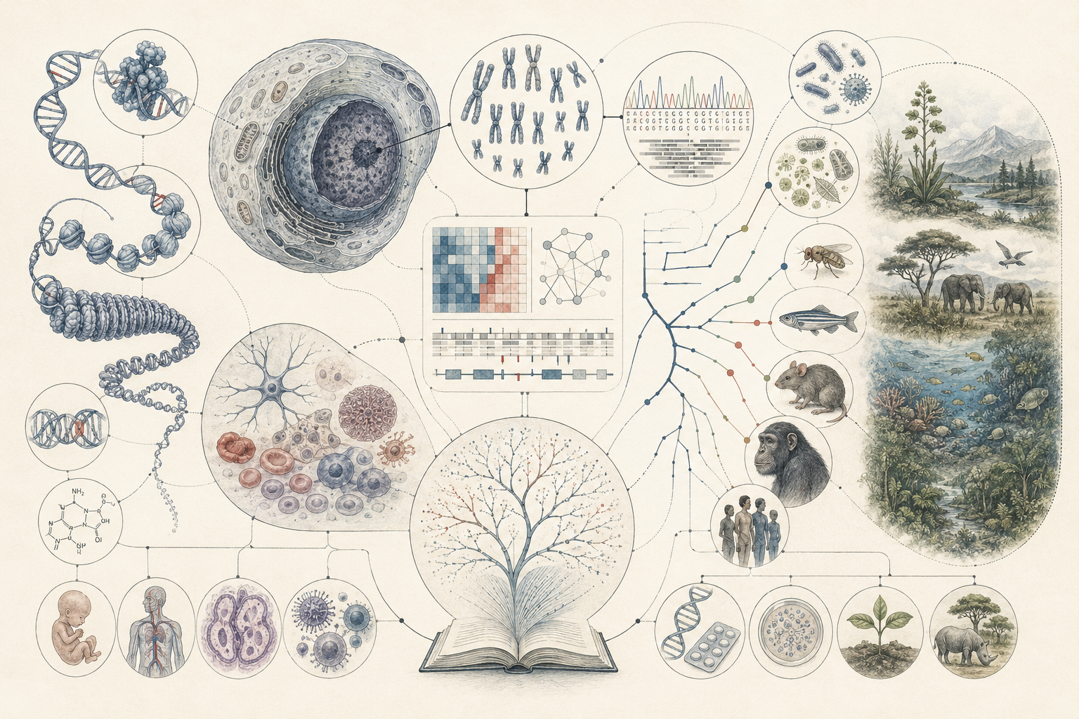
Genomics and the expansion of biological knowledge examine how the large-scale study of genomes has transformed biology from the analysis of individual genes into a broader science of whole genetic systems, regulatory architecture, variation, function, ecological response, disease, biodiversity, and evolutionary history. Genomics is one of the central developments of modern biology because it allows researchers to study not only isolated hereditary units, but also the organization, interaction, and interpretation of genetic information across organisms, populations, ecosystems, and lineages. Genomic reasoning expands biology by making whole genetic systems available for analysis: coding and noncoding sequence, chromosomal structure, regulatory landscapes, structural variation, population diversity, phylogenetic history, metagenomic community structure, and the computational systems needed to interpret them.
This article develops Genomics and the Expansion of Biological Knowledge as a foundational article within the Biology knowledge series. It treats genomics not merely as large-scale genetics, but as a change in biological scale, method, evidence, and interpretation. Genetics explains inheritance and trait transmission; genomics expands the frame to whole genomes, genome architecture, regulatory landscapes, population structure, comparative history, functional annotation, expression systems, ecological communities, disease surveillance, conservation planning, and computational inference. In that sense, genomics has not simply added more data to biology. It has changed what biology can see.
Main Library
Publications
Article Map
Biology
Related Topic
Chemistry
Related Topic
Earth Science
Related Topic
Environmental Science
The article develops genomics as a scale-spanning framework for understanding whole-genome sequencing, genome assembly, annotation, comparative genomics, functional genomics, transcriptomics, population genomics, structural variation, conservation genomics, metagenomics, pathogen genomics, plant and microbial genomics, biomedical genomics, ecological monitoring, bioinformatics, and computational biological infrastructure.
The article is written for genomic scientists, molecular biologists, computational biologists, bioinformaticians, ecologists, conservation practitioners, medical and public-health readers, plant and microbial researchers, marine and freshwater scientists, disease ecologists, biotechnology teams, and systems biologists who need a rigorous account of how genome-scale evidence expands biological knowledge across organisms, populations, communities, and environments.
The article also extends genomics into quantitative and computational biology through allele-frequency reasoning, heterozygosity, nucleotide diversity, \(F_{ST}\)-style population structure, expression fold change, sequence distance, Jukes-Cantor correction, variant-matrix quality summaries, expression-matrix summaries, PCA-style ordination, metagenomic abundance profiles, functional-potential scoring, R workflows, Python workflows, SQL provenance structures, and a linked full-stack GitHub repository containing Python, R, Julia, Fortran, Rust, Go, C, C++, SQL, notebooks, data files, validation notes, and reproducibility documentation.
What Genomics Is
Genomics is the study of the complete set of genetic material in an organism, population, community, or environmental sample, including genome structure, function, mapping, variation, regulation, interaction, and evolution. In its most useful scientific sense, genomics is not merely “genetics at larger scale.” It is a shift in biological reasoning from individual hereditary units toward whole genomes as structured, variable, regulated, historically evolving, and computationally analyzable systems.
This distinction matters because gene-centered biology can explain many aspects of inheritance and function, but it cannot by itself capture genome architecture, large-scale regulatory interaction, repetitive sequence, chromosomal organization, noncoding elements, structural variation, genome-wide expression, metagenomic community structure, or the full informational landscape through which biological systems operate. Genomics therefore expands biological knowledge by making whole genetic systems available for investigation rather than only individual loci in isolation.
In this sense, genomics is one of the clearest examples of biology becoming simultaneously more molecular, more computational, and more integrative. It allows researchers to ask how whole genomes are organized, how genomic variation is distributed across individuals and populations, how regulatory landscapes shape expression, how genomes change through evolutionary time, and how genome-scale patterns illuminate ecology, disease, adaptation, conservation, agriculture, and biological complexity.
Genomics also changes the evidentiary standard of modern biology. A biological question can now be approached through sequence data, variant calls, expression matrices, chromatin maps, metagenomic profiles, comparative alignments, phylogenomic trees, and genome-scale annotations. These data do not answer biological questions automatically, but they dramatically expand the range of questions that can be asked with precision.
From Genetics to Genomics
Classical genetics focused primarily on inheritance, trait transmission, and the roles of individual genes or loci. It asked how traits are passed from parents to offspring, how alleles segregate, how linkage modifies inheritance, and how variation shapes populations. Genomics emerged when technologies made it possible to sequence, map, compare, and analyze whole genomes. This transition widened the scope of biology in at least three major ways: it revealed that large portions of genomic organization cannot be understood through single-gene logic alone, it made large-scale comparison possible across species and populations, and it transformed biology into a far more data-intensive science.
This matters because genomics is not just an accumulation of more sequence. It changes what counts as explanation. Instead of asking only how one gene affects one trait, biology can ask how large regulatory systems coordinate activity, how chromosomal context shapes function, how structural variation reorganizes genomes, how regulatory elements influence expression, how variants interact across many loci, and how interacting genomic elements contribute to development, physiology, disease, adaptation, and environmental response.
The importance of genomics therefore lies not only in new data, but in new explanatory reach. Biology can now investigate heredity, regulation, variation, lineage history, adaptation, disease, and systems-level organization at scales that were previously inaccessible. Genomics expands the biological imagination from isolated parts toward structured systems of inherited information.
This shift also changes the relationship between biology and computation. Genetics could be mathematical long before genomics, but genomics makes computation unavoidable. Whole-genome assemblies, sequence alignments, variant matrices, transcriptomes, phylogenomic datasets, and metagenomic profiles require pipelines, statistical reasoning, data provenance, quality control, and reproducible code. Genomics is therefore both a biological science and an information science.
Genomes as Biological Systems
A genome is not merely a list of genes. It is an organized biological system containing coding sequences, noncoding regions, repetitive elements, structural features, regulatory motifs, chromosomal architecture, mobile elements, centromeres, telomeres, copy-number variation, gene families, conserved regions, and evolutionary traces. Modern genomics treats the genome as both an informational archive and an active biological substrate whose organization affects function.
This is one reason genomics changes how biology understands heredity. Hereditary information is not stored only in isolated functional units. It is embedded in larger genomic contexts that influence accessibility, expression, interaction, recombination, repair, mutation, and stability. Genome organization therefore helps shape what genes can do, when they are expressed, how they respond to developmental and environmental conditions, and how they participate in larger biological systems.
Thinking genomically encourages systems-level reasoning. It helps biology move from trait-by-trait explanation toward integrated views of sequence, architecture, regulation, interaction, variation, and history. In practice, the genome must be understood as a structured field of potential whose meaning depends on context as much as content.
This does not mean every region of a genome has the same functional meaning. Some regions encode proteins, some regulate expression, some have structural roles, some are repetitive, some are mobile, some are conserved, some are lineage-specific, and some may have uncertain or context-dependent significance. Genomic interpretation therefore requires caution. A genome is rich with biological signal, but the existence of sequence does not automatically imply a known function.
Sequencing and the Large-Scale Reading of Life
Genome sequencing transformed biology because it made it possible to read genetic information at unprecedented scale. Once genomes can be sequenced, they can be aligned, assembled, annotated, searched for variants, linked to expression patterns, compared across species, and interpreted computationally. This allows biology to move beyond identifying single genes toward large-scale analysis of genomic structure and variation.
Sequencing also changes what counts as evidence. Sequence data can now complement microscopy, physiology, field observation, ecology, experimental manipulation, clinical records, conservation monitoring, and biotechnology workflows. Genomics is therefore one of the clearest places where biology becomes both more molecular and more computational at the same time. The sequence is not the interpretation, but it creates the substrate for interpretation at a scale that earlier biology could not access.
The result is not simply a larger archive of hereditary information. It is a new capacity to ask biological questions at the level of complete genomes, multi-sample datasets, cross-lineage comparisons, and ecosystem-scale molecular surveys. In that sense, sequencing is not the end point of genomics but the entry point into a much wider analytic system.
Sequencing also brings methodological responsibility. Read length, sequencing depth, error profiles, coverage distribution, platform choice, contamination, library preparation, sample preservation, reference bias, and computational filtering can all influence genomic conclusions. A sequence dataset is therefore both biological evidence and a technical product. Strong genomic science requires documenting how the data were generated, processed, filtered, interpreted, and preserved.
Assembly, Annotation, and the Making of Genome Knowledge
Genomic knowledge is produced through assembly, annotation, quality control, comparison, and interpretation. Sequencing reads do not automatically become biological insight. They must be assembled into contiguous representations, checked for coverage and quality, annotated for genes and regulatory features, compared against known databases, and interpreted in relation to biological questions.
This matters because genomes are not discovered in finished form. They are reconstructed through computational and experimental workflows. Assembly quality, reference bias, sequencing technology, repeat structure, contamination, annotation criteria, and database limitations all shape what can be inferred. A genome sequence is therefore both a biological object and an analytical product.
Annotation is especially important because it connects raw sequence to biological meaning. Genes, transcripts, regulatory elements, repeats, structural variants, conserved regions, functional domains, and noncoding features become visible through annotation. But annotation is provisional and evidence-dependent. As new data accumulate, genome interpretation changes. Genomics is therefore not a static archive but a continuing knowledge-production system.
This is especially important outside model organisms. In well-studied systems, annotation benefits from extensive experimental knowledge, curated databases, and comparative evidence. In non-model organisms, rare species, environmental samples, or understudied ecosystems, annotation may be uncertain, incomplete, or biased toward known organisms. Genomic knowledge therefore often reflects not only biology, but also historical patterns of research investment.
Comparative Genomics and Evolutionary Knowledge
Comparative genomics studies the similarities and differences among genomes across individuals, populations, and species. It is powerful because it reveals conservation, divergence, duplication, rearrangement, horizontal transfer, lineage-specific change, introgression, gene-family expansion, and shared evolutionary history at large scale. Shared sequence can signal ancestry or conserved function. Divergent sequence can signal drift, selection, ecological specialization, altered regulatory architecture, or lineage-specific innovation.
This comparative perspective deepens evolutionary biology by showing how genomes preserve traces of common ancestry while also recording divergence, adaptation, and novelty. Large-scale comparison therefore connects genomics directly to phylogeny, functional conservation, evolutionary history, and the biological interpretation of variation.
Comparative genomics also broadens the unit of comparison in biology. Species are no longer compared only through anatomy, morphology, physiology, or ecology, but also through whole-genome organization and sequence-scale pattern. The result is a more historically grounded and more quantitatively explicit account of biological similarity and difference.
This has major implications for the tree of life. Genomics can clarify relationships that morphology alone leaves ambiguous, detect cryptic diversity, reveal hybridization or introgression, and expose horizontal gene transfer in microbial systems. It also shows that evolutionary history is not always a simple branching diagram. Genomes may carry traces of recombination, gene flow, endosymbiosis, duplication, loss, and transfer, all of which complicate but enrich evolutionary interpretation.
Functional Genomics, Regulation, and Expression
Functional genomics asks how genomes operate in living systems rather than only how they are structured. This includes the study of transcription, expression patterning, chromatin accessibility, regulatory elements, noncoding RNA, epigenetic state, protein interaction, genome-wide perturbation, and other processes that shape phenotype and function.
This matters because genomes do not act as static archives. They are interpreted dynamically through cells, tissues, developmental stages, physiological states, and environmental conditions. Functional genomics therefore shifts attention from what is present in the genome to what becomes active, when, where, and under what regulatory constraints.
In this way, genomics strengthens rather than replaces molecular biology. It allows researchers to study expression and regulation not just gene by gene, but across entire systems of coordinated activity. Genome function becomes a problem of integrated networks, not only isolated loci. Transcriptomics, epigenomics, proteomics, metabolomics, and systems biology all extend this functional-genomic logic.
Functional genomics is especially important because many biological differences are regulatory rather than strictly coding. Two organisms, tissues, or disease states may differ not only in which genes they possess, but in how those genes are regulated. Expression timing, intensity, tissue specificity, chromatin state, enhancer activity, and transcript stability can all shape biological outcome. Genomics therefore broadens biology from sequence content to sequence use.
Population Genomics, Variation, and Structure
Population genomics extends genomic analysis to variation within and among populations. It asks how alleles, haplotypes, structural variants, and genome-wide diversity are distributed across landscapes, ecological gradients, demographies, and evolutionary histories. This makes genomics central to adaptation, migration, fragmentation, introgression, local differentiation, demographic reconstruction, and conservation planning.
This matters because many important biological questions are not about one genome alone, but about the patterned distribution of genomic diversity across many genomes. Population genomics allows biology to estimate genetic structure, infer bottlenecks, identify candidate regions under selection, detect admixture, measure inbreeding, compare lineage histories, and assess adaptive potential at much finer resolution than older marker-limited approaches allowed.
Population genomics is therefore one of the strongest bridges between evolutionary biology, ecology, conservation, and data science. It connects genome-scale difference to the historical and environmental processes that produce it. It also helps reveal hidden structure that may be invisible from morphology or abundance alone.
This matters practically. A species may appear abundant across a landscape but contain highly structured populations that should not be managed as one homogeneous unit. A declining population may retain individuals but lose genomic diversity. A restored population may require not only habitat protection but also genomic representation. Population genomics helps make such hidden biological realities visible.
Structural Variation, Repeats, and Noncoding Genomic Space
Genomics has also expanded biological knowledge by making visible forms of variation that older gene-centered models often underemphasized. Single-nucleotide variants are important, but genomes also vary through insertions, deletions, duplications, inversions, translocations, copy-number changes, mobile elements, repeat expansions, and large-scale chromosomal rearrangements. These structural changes can influence gene dosage, regulation, recombination, genome stability, disease risk, adaptation, and reproductive isolation.
Repetitive and noncoding genomic regions are also central to modern interpretation. Some noncoding regions regulate gene expression, some contribute to chromosomal structure, some contain mobile elements, some influence recombination, some are conserved, and some remain poorly understood. Genomics therefore forces biology to move beyond an overly narrow view in which genomes are treated mainly as protein-coding catalogs.
This does not mean all noncoding or repetitive sequence should be casually labeled functional. Instead, it means that genome organization, regulation, and evolution cannot be understood by coding sequence alone. Modern genomics must distinguish between biochemical activity, evolutionary conservation, regulatory function, structural role, neutral variation, and unresolved biological significance.
This distinction is one of genomics’ most important intellectual contributions. It expands the field of inquiry while also requiring careful interpretation. Genome-scale data reveal more of the biological landscape, but they also demand stronger standards for evidence, function, causality, and context.
Genomics in Physiology, Development, and Biological Function
Genomics matters for physiology and development because biological function depends on large-scale patterns of expression, regulation, variation, and coordination across genomes. A tissue type, developmental trajectory, stress response, immune state, metabolic condition, or physiological adaptation often reflects not one isolated gene but the combined activity of many loci interacting across pathways and regulatory systems.
Development makes this especially clear. The emergence of tissues, organs, and body plans depends on genome-scale regulatory programs interpreted differently across space and time. Physiology likewise depends on coordinated expression of enzymes, receptors, transporters, signaling components, structural proteins, and regulatory molecules whose activity is genomically organized.
Genomics therefore helps biology connect heredity to function at a broader scale. It explains not only what genes exist, but how genome-wide systems contribute to living organization, developmental plasticity, physiological response, and functional specialization across cell types and organisms.
This has transformed how researchers study complex traits. Height, metabolic response, disease susceptibility, drought tolerance, flowering time, immune activation, stress resilience, and ecological adaptation are often distributed across many genomic regions. Genomics allows scientists to study these distributed patterns without forcing every trait into a single-gene framework.
Ecology, Conservation, and Sustainability-Adjacent Biology
Genomics is increasingly central to ecology and sustainability-adjacent biology because environmental response, adaptation, resilience, and vulnerability all have genomic dimensions. Population decline, fragmentation, inbreeding, adaptive capacity, stress tolerance, and response to climate change can often be studied more precisely when genome-scale variation is available.
Conservation biology especially benefits from genomics because genome-scale data can illuminate population structure, effective diversity, demographic history, hybridization, bottlenecks, inbreeding, local adaptation, and evolutionary potential. This makes genomics valuable not only for academic description but for long-horizon stewardship and biodiversity protection.
This matters for sustainability because species and ecosystems under stress do not merely lose abundance. They may also lose genomic diversity, adaptive flexibility, and long-term resilience. Genomics helps make those risks more visible and more analytically tractable. It provides one way to measure not only what remains, but what biological possibility remains.
This is especially important in the context of climate change, habitat fragmentation, pollution, ocean warming, freshwater stress, land-use change, disease emergence, and biodiversity loss. Genomics can help identify populations with unique adaptive variation, monitor genetic erosion, detect hidden population structure, track pathogen evolution, and support restoration planning. It does not replace ecological fieldwork, but it strengthens ecological interpretation by revealing molecular and historical dimensions that may otherwise remain invisible.
Marine, Freshwater, Soil, Plant, and Microbial Relevance
Marine biology has become increasingly genomic because marine microbes, plankton, corals, fishes, invertebrates, and symbiotic systems often require genomic tools to understand diversity, adaptation, and environmental response. Salinity stress, acidification, thermal change, oxygen limitation, pathogen exposure, and symbiosis all leave signatures in genomes and gene-expression systems that can be studied at scale.
Freshwater biology faces similar opportunities in lakes, rivers, wetlands, and sediments, where population structure, pollutant response, microbial turnover, eutrophication, habitat fragmentation, invasive species, and hydrologic change can be examined genomically. Freshwater genomics can reveal hidden biodiversity, population fragmentation, adaptive variation, pathogen presence, and community shifts that may not be visible through morphology alone.
Soil biology and microbiology are especially genomics-rich because microbial communities are diverse, often difficult to culture comprehensively, and deeply involved in decomposition, nutrient cycling, carbon turnover, nitrogen transformation, plant-microbe interaction, disease suppression, and ecosystem resilience. Metagenomics and related approaches allow researchers to study community composition and functional potential without requiring every organism to be isolated in culture.
Plant science and agroecology likewise depend strongly on genomics. Crop improvement, disease resistance, drought tolerance, nutrient-use efficiency, restoration planting, forestry resilience, seed systems, and sustainable agriculture increasingly rely on genome-scale analysis. In these fields, genomics connects heredity to environmental performance under conditions that matter directly for food systems, land systems, biodiversity, and sustainability.
Medical, Biomedical, and Disease Ecology Relevance
Genomics is foundational to medicine and biomedicine because disease risk, drug response, cancer biology, rare-disease diagnosis, pathogen evolution, and therapeutic targeting increasingly depend on genome-scale analysis. Whole-genome and related large-scale sequencing approaches widened medicine beyond single-gene disorders toward more complex patterns of susceptibility, structural variation, ancestry-informed analysis, somatic change, and pharmacogenomic relevance.
This does not eliminate classical genetics, but it widens the framework considerably. Genomics changed biomedicine because it made it possible to look beyond isolated loci toward system-level explanation of variation, regulation, and disease mechanism. Cancer genomics, rare-disease genomics, pharmacogenomics, pathogen sequencing, population-scale biobanks, and precision medicine all reflect this expanded framework.
Disease ecology adds further scale. Pathogens evolve genomically, hosts vary genomically, and populations interact under ecological pressures that shape selection and spread. Genomics therefore connects molecular change to clinical and epidemiological consequence. It is one of the main reasons modern disease surveillance can track variants, outbreaks, transmission pathways, and evolutionary change with far greater resolution than older tools allowed.
This is especially relevant for antimicrobial resistance, viral evolution, zoonotic spillover, vector-borne disease, hospital outbreaks, wastewater surveillance, and global pathogen monitoring. Genomics does not remove the need for clinical, social, ecological, and public-health context, but it gives disease science a powerful way to identify lineage, transmission, adaptation, and resistance at molecular resolution.
Biotechnology, Bioinformatics, and Computational Relevance
Genomics is one of the clearest places where biology and computation become inseparable. Whole genomes generate far more information than can be interpreted without computational tools. Sequence assembly, alignment, annotation, variant calling, transcriptomic analysis, phylogenomics, metagenomic inference, population-structure analysis, and increasingly machine-assisted interpretation all depend on bioinformatics and computational biology.
Biotechnology depends on this computational infrastructure because genomics informs sequencing workflows, diagnostics, breeding, strain verification, synthetic biology, environmental monitoring, biomarker discovery, cell-line characterization, pathway engineering, and reproducible biological data systems. In biotechnology, genomes become not only objects of explanation but also resources for design, classification, and intervention.
This makes genomics one of the strongest bridges between basic biology and applied scientific systems. It is both a knowledge framework and an operating infrastructure, and its scientific value depends increasingly on rigorous quantitative interpretation, careful provenance, reproducible computation, transparent analytical assumptions, and biological validation.
Genomics also illustrates why data governance matters in science. A genomic dataset is not just a file. It carries information about organisms, populations, environments, health, ancestry, pathogens, ecosystems, and sometimes human communities. Good genomic science therefore requires not only technical rigor, but also ethical care about consent, privacy, benefit sharing, Indigenous data sovereignty where relevant, conservation implications, clinical interpretation, and responsible use.
Mathematical lens
Genomics is inherently quantitative because genome-scale analysis depends on counting, comparing, aligning, estimating, and modeling large bodies of sequence, expression, and variation data. This does not reduce genomics to computation alone, but it does mean that mathematics, statistics, and programming are built into the discipline at a deep level.
At a biallelic locus, a basic allele-frequency relation is:
Interpretation: In a simple two-allele model, the two allele frequencies sum to one.
where \(p\) and \(q\) are allele frequencies. Under Hardy-Weinberg assumptions, expected genotype frequencies are:
Interpretation: Genotype expectations are determined from allele frequencies under idealized population assumptions.
This remains useful in genomics because many genomic analyses still begin with variation frequencies, genotype expectations, and departures from those expectations.
A standard biallelic diversity measure is expected heterozygosity:
Interpretation: Expected heterozygosity summarizes standing genetic variation at a biallelic locus.
This is useful because genomic diversity is often summarized not just by which allele is common, but by how much variation remains in the population.
Across many biallelic sites, a simple nucleotide-diversity approximation is:
Interpretation: Nucleotide diversity summarizes average variation across many genomic sites.
where \(L\) is the number of sites and \(p_i\) is the allele frequency at site \(i\). This is useful because genome-scale diversity is usually a multi-locus property rather than a one-locus property.
A fixation-style summary for population differentiation is:
Interpretation: \(F_{ST}\)-style summaries estimate how much genetic variation is partitioned among populations relative to total variation.
where \(H_T\) is total expected heterozygosity and \(H_S\) is mean within-population heterozygosity. This is useful because genomics frequently asks how much variation is partitioned within versus among populations.
A common measure of expression change between two conditions is:
Interpretation: Log2 fold change expresses expression differences on a symmetric scale.
where \(E_1\) and \(E_2\) are expression levels in two different conditions and \(\epsilon\) is a small pseudocount. This is useful because genomics frequently compares transcript abundance across tissues, treatments, genotypes, disease states, or environmental conditions.
A basic observed sequence difference between equal-length strings can be written as:
Interpretation: Observed sequence distance is the fraction of aligned positions that differ.
where \(m\) is the number of mismatches and \(L\) is sequence length. A Jukes-Cantor correction is:
Interpretation: Jukes-Cantor correction adjusts observed distance for hidden substitutions under a simple evolutionary model.
This is useful because observed mismatch counts can underestimate deeper divergence when multiple substitutions affect the same sites across time.
For a metagenomic or community sample, relative abundance can be written as:
Interpretation: Relative abundance estimates the share of reads or observations assigned to taxon or feature \(i\).
where \(r_i\) is the read count assigned to taxon or feature \(i\). This is useful because environmental genomics often studies communities rather than single organisms.
Variables, Units, and Genomic Interpretation
Quantitative genomics depends on variables that connect alleles, variants, sequences, expression matrices, population structure, genomic distance, metagenomic abundance, and biological interpretation. The table below summarizes several central quantities.
| Symbol or Term | Meaning | Typical Unit or Scale | Genomic Interpretation |
|---|---|---|---|
| \(p, q\) | Allele frequencies | fraction from 0 to 1 | Relative frequency of alleles in a population or sample |
| \(p^2, 2pq, q^2\) | Genotype expectations | frequency or probability | Expected genotype frequencies under idealized assumptions |
| \(H_e\) | Expected heterozygosity | fraction from 0 to 1 | Expected fraction of heterozygotes or compact diversity measure |
| \(\pi\) | Nucleotide diversity | average differences per site or diversity fraction | Genome-scale summary of sequence variation across sites |
| \(L\) | Number of sites or sequence length | base pairs, nucleotides, loci, or aligned positions | Genomic length or number of positions being analyzed |
| \(p_i\) | Allele frequency at site \(i\) | fraction from 0 to 1 | Site-specific allele frequency used in multi-locus summaries |
| \(F_{ST}\) | Population differentiation summary | dimensionless fraction-like statistic | Degree to which variation is partitioned among populations |
| \(H_T\) | Total expected heterozygosity | fraction from 0 to 1 | Diversity expected in the combined population |
| \(H_S\) | Mean within-population heterozygosity | fraction from 0 to 1 | Average diversity within subpopulations |
| \(E_1, E_2\) | Expression values in two conditions | counts, normalized counts, TPM, FPKM, or assay units | Expression levels being compared across samples or conditions |
| \(\epsilon\) | Pseudocount | same as expression value | Small value used to avoid division by zero in fold-change calculations |
| \(\log_2FC\) | Log2 fold change | log2 ratio | Symmetric measure of expression change between conditions |
| \(d\) | Observed sequence distance | fraction from 0 to 1 | Share of aligned positions with mismatches |
| \(d_{\mathrm{JC}}\) | Jukes-Cantor corrected distance | substitutions per site under a simple model | Corrected molecular distance accounting for hidden substitutions |
| \(m\) | Mismatch count | count | Number of differing positions between aligned sequences |
| \(r_i\) | Read count for feature \(i\) | count | Number of reads assigned to a taxon, gene, feature, or functional category |
| \(a_i\) | Relative abundance | fraction from 0 to 1 | Share of reads or observations assigned to feature \(i\) |
| Missingness | Fraction of missing genotype calls | fraction from 0 to 1 | Quality-control measure in variant matrices |
| MAF | Minor allele frequency | fraction from 0 to 0.5 | Frequency of the less common allele at a variant site |
The table shows why genomic quantities require context. An allele frequency, \(F_{ST}\)-style statistic, expression fold change, sequence distance, or metagenomic abundance value becomes biologically meaningful only when linked to sampling design, organism, population, environment, reference genome, normalization method, and analytical pipeline.
Worked Example: Genotype Diversity, Distance, and Expression Change
Suppose allele \(A\) has frequency \(p=0.8\). Then:
Interpretation: In a biallelic model, the second allele frequency is determined once the first is known.
Expected genotype frequencies are:
Interpretation: The expected homozygous \(AA\) frequency is 0.64 under idealized assumptions.
Interpretation: The expected heterozygous frequency is 0.32.
Interpretation: The expected homozygous \(aa\) frequency is 0.04.
Expected heterozygosity is:
Interpretation: The expected heterozygosity at this locus is 0.32.
This is useful because it turns genomic variation into interpretable population expectations.
Sequence comparison can be analyzed similarly. Suppose two equal-length sequences have 4 mismatches across 40 aligned positions:
Interpretation: The observed sequence distance is 0.10, meaning 10 percent of aligned positions differ.
A Jukes-Cantor correction gives:
Interpretation: The corrected distance is slightly larger because it accounts for possible hidden substitutions.
This is useful because comparative genomics often begins with observed difference but must consider deeper evolutionary divergence.
Expression change provides another common genomic calculation. If a transcript has mean expression of \(E_1=40\) in a control condition and \(E_2=160\) in a treated condition, then:
Interpretation: A fourfold increase corresponds to a log2 fold change of 2.
This is useful because log2 fold change makes increases and decreases easier to compare across genes, samples, treatments, and environmental states.
Computational modeling
Computational modeling helps make genomics explicit because genomic evidence is large-scale, structured, and model-dependent. Variant matrices must be summarized through allele frequency, missingness, heterozygosity, and quality metrics. Expression matrices must be normalized, compared, reduced, and interpreted across samples. Population structure requires multi-locus reasoning. Sequence comparison requires distance calculations and model assumptions. Metagenomic data require abundance summaries, feature assignment, and functional interpretation.
The selected examples below focus on compact, reusable workflows: expression matrices, log2 fold change, PCA-style ordination, multi-locus diversity, \(F_{ST}\)-style population structure, pairwise sequence-distance matrices, variant-matrix quality summaries, minor allele frequency, missingness, heterozygosity, metagenomic abundance, and functional-potential scoring. The GitHub repository extends the same logic into richer workflows for SQL provenance, reproducible data files, validation notes, notebooks, and multi-language scientific-computing examples.
The purpose is not to reduce genomics to code. The purpose is to make genomic evidence inspectable. A genomic claim becomes stronger when sequence sources, variant filters, expression normalization, sample metadata, quality-control decisions, model assumptions, and code are documented together.
R workflow: expression, diversity, population structure, and sequence distance
R is useful for genomics because it supports statistical modeling, matrix summaries, expression analysis, population-genetic summaries, reproducible reporting, and exploratory ordination. The following workflow simulates a compact expression matrix, estimates log2 fold change, creates a PCA-style scaffold, estimates multi-locus diversity and \(F_{ST}\)-style structure, and builds a pairwise sequence-distance table.
# Genomics and the Expansion of Biological Knowledge Workflow
#
# This workflow demonstrates four quantitative genomics tasks:
#
#   1. Summarize a genome-scale expression matrix.
#   2. Calculate log2 fold change and PCA-style sample structure.
#   3. Estimate multi-locus diversity and FST-style population structure.
#   4. Build a pairwise sequence-distance table and matrix.
#
# These examples can be adapted for transcriptomics, conservation genomics,
# population genomics, comparative genomics, plant genomics, disease genomics,
# ecological monitoring, and computational biology.

library(dplyr)
library(tidyr)
library(purrr)
library(stringr)
library(tibble)

# ------------------------------------------------------------
# 1. Expression matrix, log2 fold change, variance, and PCA
# ------------------------------------------------------------

set.seed(42)

genes <- paste0("gene_", 1:200)
samples <- paste0("sample_", 1:8)
group <- c(rep("control", 4), rep("treated", 4))

expr_mat <- matrix(
  rpois(200 * 8, lambda = 100),
  nrow = 200,
  ncol = 8,
  dimnames = list(genes, samples)
)

# Add synthetic treatment-responsive structure.
expr_mat[1:15, 5:8] <- expr_mat[1:15, 5:8] + 60
expr_mat[16:30, 5:8] <- pmax(expr_mat[16:30, 5:8] - 35, 1)

expr_df <- as.data.frame(expr_mat) %>%
  tibble::rownames_to_column("gene")

meta_df <- tibble(
  sample = samples,
  group = group
)

long_df <- expr_df %>%
  pivot_longer(-gene, names_to = "sample", values_to = "count") %>%
  left_join(meta_df, by = "sample")

summary_df <- long_df %>%
  group_by(gene, group) %>%
  summarise(
    mean_count = mean(count),
    var_count = var(count),
    .groups = "drop"
  ) %>%
  pivot_wider(names_from = group, values_from = c(mean_count, var_count)) %>%
  mutate(
    log2_fc = log2((mean_count_treated + 1) / (mean_count_control + 1)),
    mean_expression = (mean_count_treated + mean_count_control) / 2
  ) %>%
  arrange(desc(abs(log2_fc)))

log_expr <- log2(expr_mat + 1)
pca <- prcomp(t(log_expr), center = TRUE, scale. = TRUE)

pca_df <- as.data.frame(pca$x[, 1:2]) %>%
  tibble::rownames_to_column("sample") %>%
  left_join(meta_df, by = "sample")

# ------------------------------------------------------------
# 2. Multi-locus diversity and FST-style structure
# ------------------------------------------------------------

set.seed(7)

loci <- 1000
p_anc <- runif(loci, 0.05, 0.95)

n1 <- 200
n2 <- 80

p1 <- rbinom(loci, size = n1, prob = p_anc) / n1
p2 <- rbinom(loci, size = n2, prob = p_anc) / n2

geno_df <- tibble(
  locus = 1:loci,
  p1 = p1,
  p2 = p2
) %>%
  mutate(
    pi1 = 2 * p1 * (1 - p1),
    pi2 = 2 * p2 * (1 - p2),
    pbar = (p1 + p2) / 2,
    HT = 2 * pbar * (1 - pbar),
    HS = (pi1 + pi2) / 2,
    fst = ifelse(HT > 0, (HT - HS) / HT, 0),
    delta_p = abs(p1 - p2)
  )

population_summary <- geno_df %>%
  summarise(
    mean_pi1 = mean(pi1),
    mean_pi2 = mean(pi2),
    mean_fst = mean(fst),
    mean_delta_p = mean(delta_p)
  )

# ------------------------------------------------------------
# 3. Pairwise sequence distance and exploratory clustering
# ------------------------------------------------------------

seqs <- c(
  genome_A = "ATGCTAGCTAACGGTACCTA",
  genome_B = "ATGCTGGCTATCGGTACCTA",
  genome_C = "ATGATGGCTATCGGTTCCTA",
  genome_D = "ATGCTAGTTAACGGAACCTG",
  genome_E = "ATGCTAGCTAACGGAACCTA"
)

pair_dist <- function(s1, s2) {
  x <- str_split(s1, "", simplify = TRUE)
  y <- str_split(s2, "", simplify = TRUE)

  mismatches <- sum(x != y)
  L <- length(x)
  p <- mismatches / L

  jc <- ifelse(
    p >= 0.75,
    NA_real_,
    -(3 / 4) * log(1 - (4 / 3) * p)
  )

  tibble(
    mismatches = mismatches,
    p_distance = p,
    jukes_cantor = jc
  )
}

pairs <- expand.grid(
  seq1 = names(seqs),
  seq2 = names(seqs),
  stringsAsFactors = FALSE
) %>%
  as_tibble() %>%
  filter(seq1 < seq2) %>%
  mutate(res = map2(seq1, seq2, ~ pair_dist(seqs[[.x]], seqs[[.y]]))) %>%
  unnest(res)

taxa <- names(seqs)

dist_mat <- matrix(
  0,
  nrow = length(taxa),
  ncol = length(taxa),
  dimnames = list(taxa, taxa)
)

for (i in seq_len(nrow(pairs))) {
  a <- pairs$seq1[i]
  b <- pairs$seq2[i]

  dist_mat[a, b] <- pairs$jukes_cantor[i]
  dist_mat[b, a] <- pairs$jukes_cantor[i]
}

hc <- hclust(as.dist(dist_mat), method = "average")

print(summary_df %>% slice_head(n = 20))
print(pca_df)

print(round(population_summary, 4))
print(geno_df %>% arrange(desc(fst)) %>% slice_head(n = 20) %>% mutate(across(where(is.numeric), round, 4)))

print(pairs)
print(round(dist_mat, 4))
print(hc)
This R workflow is useful because genome-scale reasoning rarely stops at one statistic. Researchers often need expression matrices, variance summaries, sample-level ordination, multi-locus population structure, sequence distances, and exploratory comparisons in one reproducible workflow.
Python workflow: variant matrices, population structure, sequence distance, and metagenomics
Python is useful for genomics because it supports matrix analysis, simulation, pipeline design, sequence comparison, quality-control summaries, numerical computation, and reproducible data workflows. The following workflow summarizes variant matrices, estimates minor allele frequency and heterozygosity, calculates population-structure scaffolds, builds pairwise sequence-distance matrices, and summarizes metagenomic abundance and functional potential.
"""
Genomics and the Expansion of Biological Knowledge Workflow

This workflow demonstrates five quantitative genomics tasks:

1. Summarize a variant matrix using allele frequency, MAF, heterozygosity,
   and missingness.
2. Build an expression matrix and PCA-style sample ordination.
3. Estimate genome-wide population-structure summaries.
4. Build pairwise sequence-distance tables and matrices.
5. Summarize metagenomic relative abundance and functional potential.

The examples are compact, but the same structures can be extended to
population genomics, comparative genomics, transcriptomics, conservation
genomics, pathogen genomics, environmental genomics, and biotechnology.
"""

from __future__ import annotations

from itertools import combinations

import numpy as np
import pandas as pd


def variant_matrix_summary(seed: int = 42) -> tuple[pd.DataFrame, pd.DataFrame]:
    """
    Simulate and summarize a diploid genotype matrix.

    Genotypes:
    0 = homozygous reference
    1 = heterozygous
    2 = homozygous alternate
    NaN = missing call
    """
    rng = np.random.default_rng(seed)

    n_individuals = 60
    n_loci = 300

    true_freqs = rng.beta(0.7, 2.5, size=n_loci)
    genotype_matrix = rng.binomial(
        2,
        true_freqs,
        size=(n_individuals, n_loci),
    ).astype(float)

    missing_mask = rng.random(size=genotype_matrix.shape) < 0.03
    genotype_matrix[missing_mask] = np.nan

    geno = pd.DataFrame(genotype_matrix)

    alt_freq = geno.mean(axis=0, skipna=True) / 2.0
    maf = np.minimum(alt_freq, 1.0 - alt_freq)

    obs_het = (geno == 1).sum(axis=0) / geno.notna().sum(axis=0)
    exp_het = 2.0 * alt_freq * (1.0 - alt_freq)
    missing_rate = geno.isna().mean(axis=0)

    summary_df = pd.DataFrame(
        {
            "alt_freq": alt_freq,
            "maf": maf,
            "obs_het": obs_het,
            "exp_het": exp_het,
            "missing_rate": missing_rate,
        }
    )

    descriptive_summary = summary_df.describe().reset_index()

    return summary_df, descriptive_summary


def expression_matrix_ordination(seed: int = 7) -> tuple[pd.DataFrame, pd.DataFrame]:
    """
    Simulate an expression matrix and build PCA-style sample scores.
    """
    rng = np.random.default_rng(seed)

    n_genes = 250
    n_samples = 10
    groups = np.array(["control"] * 5 + ["treated"] * 5)

    expr = rng.poisson(lam=100, size=(n_genes, n_samples)).astype(float)

    # Add synthetic treatment-responsive structure.
    expr[:20, 5:] += 55
    expr[20:40, 5:] = np.maximum(expr[20:40, 5:] - 30, 1)

    expr_df = pd.DataFrame(
        expr,
        columns=[f"sample_{i + 1}" for i in range(n_samples)],
    )

    control_mean = expr_df.iloc[:, :5].mean(axis=1)
    treated_mean = expr_df.iloc[:, 5:].mean(axis=1)

    gene_summary = pd.DataFrame(
        {
            "gene": [f"gene_{i + 1}" for i in range(n_genes)],
            "control_mean": control_mean,
            "treated_mean": treated_mean,
            "log2_fc": np.log2((treated_mean + 1.0) / (control_mean + 1.0)),
        }
    ).sort_values("log2_fc", ascending=False)

    log_expr = np.log2(expr_df + 1.0)

    x = log_expr.sub(log_expr.mean(axis=1), axis=0).T.values
    x_centered = x - x.mean(axis=0, keepdims=True)

    u, singular_values, _ = np.linalg.svd(x_centered, full_matrices=False)
    scores = u[:, :2] * singular_values[:2]

    pca_df = pd.DataFrame(
        {
            "sample": expr_df.columns,
            "group": groups,
            "PC1": scores[:, 0],
            "PC2": scores[:, 1],
        }
    )

    return gene_summary, pca_df


def population_structure_scaffold(seed: int = 99) -> tuple[pd.DataFrame, pd.DataFrame]:
    """
    Simulate two populations and calculate diversity and FST-style summaries.
    """
    rng = np.random.default_rng(seed)

    n_loci = 500
    p_anc = rng.uniform(0.05, 0.95, size=n_loci)

    p1 = rng.binomial(150, p_anc) / 150.0
    p2 = rng.binomial(60, p_anc) / 60.0

    pbar = (p1 + p2) / 2.0
    ht = 2.0 * pbar * (1.0 - pbar)
    hs = (2.0 * p1 * (1.0 - p1) + 2.0 * p2 * (1.0 - p2)) / 2.0

    fst = np.where(ht > 0, (ht - hs) / ht, 0.0)

    df = pd.DataFrame(
        {
            "p1": p1,
            "p2": p2,
            "pi1": 2.0 * p1 * (1.0 - p1),
            "pi2": 2.0 * p2 * (1.0 - p2),
            "delta_p": np.abs(p1 - p2),
            "fst": fst,
        }
    )

    summary = pd.DataFrame(
        {
            "mean_pi1": [df["pi1"].mean()],
            "mean_pi2": [df["pi2"].mean()],
            "mean_delta_p": [df["delta_p"].mean()],
            "mean_fst": [df["fst"].mean()],
        }
    )

    return df, summary


def jukes_cantor_distance(p_distance: float) -> float:
    """
    Calculate Jukes-Cantor corrected distance from observed p-distance.
    """
    if p_distance >= 0.75:
        return float("nan")

    return float(-(3.0 / 4.0) * np.log(1.0 - (4.0 / 3.0) * p_distance))


def pairwise_distance(seq1: str, seq2: str) -> tuple[int, float, float]:
    """
    Return mismatch count, p-distance, and Jukes-Cantor distance.
    """
    if len(seq1) != len(seq2):
        raise ValueError("Sequences must be equal length for this simple example.")

    mismatches = sum(base_a != base_b for base_a, base_b in zip(seq1, seq2))
    length = len(seq1)
    p_distance = mismatches / length
    jc_distance = jukes_cantor_distance(p_distance)

    return mismatches, p_distance, jc_distance


def sequence_distance_matrix() -> tuple[pd.DataFrame, pd.DataFrame]:
    """
    Build pairwise sequence-distance table and matrix.
    """
    seqs = {
        "genome_A": "ATGCTAGCTAACGGTACCTA",
        "genome_B": "ATGCTGGCTATCGGTACCTA",
        "genome_C": "ATGATGGCTATCGGTTCCTA",
        "genome_D": "ATGCTAGTTAACGGAACCTG",
        "genome_E": "ATGCTAGCTAACGGAACCTA",
    }

    rows = []

    for taxon_a, taxon_b in combinations(seqs.keys(), 2):
        mismatches, p_distance, jc_distance = pairwise_distance(
            seqs[taxon_a],
            seqs[taxon_b],
        )

        rows.append(
            {
                "taxon_1": taxon_a,
                "taxon_2": taxon_b,
                "mismatches": mismatches,
                "p_distance": p_distance,
                "jukes_cantor": jc_distance,
            }
        )

    dist_df = pd.DataFrame(rows)

    taxa = list(seqs.keys())
    matrix = pd.DataFrame(
        np.zeros((len(taxa), len(taxa))),
        index=taxa,
        columns=taxa,
    )

    for _, row in dist_df.iterrows():
        matrix.loc[row["taxon_1"], row["taxon_2"]] = row["jukes_cantor"]
        matrix.loc[row["taxon_2"], row["taxon_1"]] = row["jukes_cantor"]

    return dist_df, matrix


def metagenomic_abundance_summary() -> pd.DataFrame:
    """
    Summarize metagenomic relative abundance and functional potential.
    """
    metagenome = pd.DataFrame(
        {
            "taxon": [
                "Nitrosomonas",
                "Pseudomonas",
                "Bacteroides",
                "Rhizobium",
                "Vibrio",
                "Bacillus",
            ],
            "reads": [12000, 8500, 6100, 4200, 1800, 3600],
            "carbon_cycle_genes": [18, 11, 7, 9, 2, 5],
            "nitrogen_cycle_genes": [21, 6, 2, 19, 1, 4],
            "stress_response_genes": [44, 39, 28, 22, 17, 31],
        }
    )

    metagenome["relative_abundance"] = (
        metagenome["reads"] / metagenome["reads"].sum()
    )

    metagenome["functional_potential_score"] = (
        0.35
        * metagenome["carbon_cycle_genes"]
        / metagenome["carbon_cycle_genes"].max()
        + 0.35
        * metagenome["nitrogen_cycle_genes"]
        / metagenome["nitrogen_cycle_genes"].max()
        + 0.30
        * metagenome["stress_response_genes"]
        / metagenome["stress_response_genes"].max()
    )

    return metagenome.sort_values(
        "functional_potential_score",
        ascending=False,
    )


def main() -> None:
    """
    Run compact genomics workflows.
    """
    variant_summary, variant_descriptive = variant_matrix_summary()
    gene_summary, pca_df = expression_matrix_ordination()
    pop_df, pop_summary = population_structure_scaffold()
    dist_df, dist_matrix = sequence_distance_matrix()
    metagenome_df = metagenomic_abundance_summary()

    print("Variant matrix summary:")
    print(variant_summary.head(20).round(4).to_string(index=False))
    print("\nVariant descriptive summary:")
    print(variant_descriptive.round(4).to_string(index=False))

    print("\nTop expression changes:")
    print(gene_summary.head(20).round(4).to_string(index=False))

    print("\nPCA-style expression ordination:")
    print(pca_df.round(4).to_string(index=False))

    print("\nPopulation structure summary:")
    print(pop_summary.round(4).to_string(index=False))
    print(pop_df.sort_values("fst", ascending=False).head(20).round(4).to_string(index=False))

    print("\nPairwise sequence-distance table:")
    print(dist_df.round(4).to_string(index=False))

    print("\nJukes-Cantor distance matrix:")
    print(dist_matrix.round(4).to_string())

    print("\nMetagenomic abundance and functional potential:")
    print(metagenome_df.round(4).to_string(index=False))


if __name__ == "__main__":
    main()
This Python workflow is useful because genomics increasingly includes population-scale, comparative, expression-level, and environmental data in the same scientific ecosystem. Variant quality, allele frequencies, sample structure, sequence distance, and metagenomic functional potential are different forms of genomic evidence that need transparent computational scaffolding.
GitHub repository
The article body includes compact R and Python examples so the biological and scientific argument remains readable. The full repository expands those examples into a broader computational genomics workflow, including expression matrices, log2 fold change, PCA-style ordination, variant-matrix summaries, minor allele frequency, heterozygosity, missingness, nucleotide diversity, \(F_{ST}\)-style population structure, sequence-distance matrices, Jukes-Cantor correction, metagenomic abundance profiles, functional-potential scoring, SQL provenance structures, reproducible data files, validation notes, and full-stack scientific-computing examples across Python, R, Julia, Fortran, Rust, Go, C, C++, SQL, and notebooks.
Limits, Complexity, and Modern Genomic Thinking
Genomics is powerful, but it does not automatically explain everything. Sequence alone does not determine all biological outcomes. Genome-scale data require interpretation, context, and connection to development, physiology, environment, ecology, evolution, disease, and experimental design. A large dataset is not a biological explanation by itself.
This is why modern genomic thinking increasingly emphasizes integration. Genomics is strongest when linked to transcriptomics, proteomics, epigenetics, physiology, ecology, population history, field observation, and careful experimental design. Genome-scale knowledge expands biological understanding, but it does not remove the need for judgment across scales.
Models and workflows are useful because they clarify assumptions, expose patterns, and make comparison possible. But a PCA plot is not a biological mechanism, a variant-frequency table is not a complete population history, and a metagenomic abundance profile is not a complete ecosystem model. Quantitative genomics is strongest when it supports biological interpretation rather than replacing it.
In that sense, genomics is a model case of modern biology: data-rich, computationally intensive, mechanistically informative, historically grounded, and yet always dependent on broader biological interpretation. Its strength lies not in raw scale alone, but in disciplined integration.
This caution is especially important because genomic tools can create false confidence. A dataset may look precise while remaining biased by sampling, reference choice, sequencing depth, annotation gaps, batch effects, population structure, contamination, or incomplete metadata. Genomics expands biological knowledge only when its technical power is paired with interpretive humility.
Why This Matters for Scientific Work
For working scientists, genomics matters because many biological questions are misread when genomes are treated as passive sequence archives rather than active, structured, variable systems. A conservation problem may hinge on hidden population structure. A disease problem may depend on structural variation or noncoding regulation rather than one obvious coding mutation. A microbial ecology problem may require metagenomic resolution to identify community turnover or metabolic potential. A plant or marine resilience problem may turn on genome-scale adaptive variation under stress.
This means genomics should often be treated as explanatory infrastructure rather than as a specialized methods layer. Molecular biologists need it because regulation operates genome-wide. Ecologists need it because response to disturbance has genomic dimensions. Conservation scientists need it because long-term persistence depends partly on genomic diversity. Biomedical scientists need it because disease risk and treatment response often involve distributed genomic factors. Computational biologists need it because genomes are among the most important large-scale structured data objects in modern science.
The scientific importance of genomics lies partly in this breadth. It is one of the principal ways biology enlarges its explanatory scope from isolated hereditary units to whole systems of variation, regulation, function, and history.
Genomics is also practically actionable. It can support variant detection, disease surveillance, biodiversity monitoring, population management, crop improvement, strain tracking, ecological restoration, outbreak investigation, environmental monitoring, and biotechnology development. Its power lies not only in reading genomes, but in connecting genome-scale evidence to decisions about living systems.
Conclusion
Genomics and the expansion of biological knowledge show that biology has moved beyond the study of isolated hereditary units toward the large-scale analysis of whole genomic systems. This shift has broadened what scientists can know about variation, regulation, function, evolution, adaptation, disease, biodiversity, and biological complexity across cells, organisms, populations, and ecosystems.
To understand genomics is therefore to understand one of the major ways modern biology has expanded its scope. Genomes are not merely containers of genes. They are large, structured, evolving systems whose analysis helps connect heredity to ecology, development, medicine, conservation, and biotechnology. That is why genomics remains central not only to molecular biology and genetics, but also to sustainability-adjacent biology across environmental and applied domains.
Genomics is thus more than a technical specialty. It is one of the principal ways biology enlarges its own field of vision. Modern quantitative and computational workflows deepen that expansion by making genomic evidence more transparent, reproducible, and interpretable across scales.
Related articles
- Biology
- DNA, RNA, and the Molecular Logic of Life
- Molecular Biology and the Flow of Genetic Information
- Genes, Inheritance, and the Principles of Heredity
- Mutation, Variation, and the Sources of Novelty
- Epigenetics, Regulation, and Gene Expression
- Population Genetics and the Mathematics of Inheritance
- Speciation, Diversity, and the Tree of Life
- Evolution and the History of Life
- Development, Differentiation, and the Making of Organisms
- Systems Biology and the Logic of Biological Integration
- Observation, Experiment, and the Methods of Biological Inquiry
Further reading
- Brown, T.A. (2002) ‘Understanding a genome sequence’, in Genomes. 2nd edn. Oxford: Wiley-Liss. Available at: https://www.ncbi.nlm.nih.gov/books/NBK21136/
- ENCODE Project Consortium (2012) ‘An integrated encyclopedia of DNA elements in the human genome’, Nature, 489, pp. 57–74. Available at: https://doi.org/10.1038/nature11247
- ENCODE Project Consortium et al. (2020) ‘Expanded encyclopaedias of DNA elements in the human and mouse genomes’, Nature, 583, pp. 699–710. Available at: https://doi.org/10.1038/s41586-020-2493-4
- Koonin, E.V. and Galperin, M.Y. (2003) ‘Genome annotation and analysis’, in Sequence – Evolution – Function: Computational Approaches in Comparative Genomics. Boston: Kluwer Academic. Available at: https://www.ncbi.nlm.nih.gov/books/NBK20253/
- National Human Genome Research Institute (n.d.) About Genomics. Available at: https://www.genome.gov/about-genomics
- National Human Genome Research Institute (n.d.) A Brief Guide to Genomics. Available at: https://www.genome.gov/about-genomics/fact-sheets/A-Brief-Guide-to-Genomics
- National Human Genome Research Institute (n.d.) Gene Expression. Available at: https://www.genome.gov/genetics-glossary/Gene-Expression
- National Human Genome Research Institute (n.d.) Genetics vs. Genomics. Available at: https://www.genome.gov/about-genomics/fact-sheets/Genetics-vs-Genomics
- National Human Genome Research Institute (n.d.) Human Genomic Variation. Available at: https://www.genome.gov/about-genomics/educational-resources/fact-sheets/human-genomic-variation
- National Human Genome Research Institute (n.d.) The Human Genome Project. Available at: https://www.genome.gov/human-genome-project
- National Research Council (1990) Mapping and Sequencing the Human Genome. Washington, DC: National Academies Press. Available at: https://www.ncbi.nlm.nih.gov/sites/books/n/nap9990/
- Saeed, U. and Abbasi, B.A. (2019) ‘Biological sequence analysis’, in StatPearls. Treasure Island, FL: StatPearls Publishing. Available at: https://www.ncbi.nlm.nih.gov/books/NBK550342/
References
- Brown, T.A. (2002) ‘Understanding a genome sequence’, in Genomes. 2nd edn. Oxford: Wiley-Liss. Available at: https://www.ncbi.nlm.nih.gov/books/NBK21136/
- ENCODE Project Consortium (2012) ‘An integrated encyclopedia of DNA elements in the human genome’, Nature, 489, pp. 57–74. Available at: https://doi.org/10.1038/nature11247
- ENCODE Project Consortium et al. (2020) ‘Expanded encyclopaedias of DNA elements in the human and mouse genomes’, Nature, 583, pp. 699–710. Available at: https://doi.org/10.1038/s41586-020-2493-4
- Koonin, E.V. and Galperin, M.Y. (2003) ‘Genome annotation and analysis’, in Sequence – Evolution – Function: Computational Approaches in Comparative Genomics. Boston: Kluwer Academic. Available at: https://www.ncbi.nlm.nih.gov/books/NBK20253/
- National Human Genome Research Institute (n.d.) A Brief Guide to Genomics. Available at: https://www.genome.gov/about-genomics/fact-sheets/A-Brief-Guide-to-Genomics
- National Human Genome Research Institute (n.d.) About Genomics. Available at: https://www.genome.gov/about-genomics
- National Human Genome Research Institute (n.d.) Gene Expression. Available at: https://www.genome.gov/genetics-glossary/Gene-Expression
- National Human Genome Research Institute (n.d.) Genetics vs. Genomics. Available at: https://www.genome.gov/about-genomics/fact-sheets/Genetics-vs-Genomics
- National Human Genome Research Institute (n.d.) Human Genomic Variation. Available at: https://www.genome.gov/about-genomics/educational-resources/fact-sheets/human-genomic-variation
- National Human Genome Research Institute (n.d.) The Human Genome Project. Available at: https://www.genome.gov/human-genome-project
- National Research Council (1990) Mapping and Sequencing the Human Genome. Washington, DC: National Academies Press. Available at: https://www.ncbi.nlm.nih.gov/sites/books/n/nap9990/
- Saeed, U. and Abbasi, B.A. (2019) ‘Biological sequence analysis’, in StatPearls. Treasure Island, FL: StatPearls Publishing. Available at: https://www.ncbi.nlm.nih.gov/books/NBK550342/