
Last Updated May 28, 2026
Population genetics and the mathematics of inheritance examine how allele frequencies change through time, how heredity operates at the level of whole populations rather than isolated pedigrees alone, and how mathematical models help explain the evolutionary consequences of selection, drift, mutation, migration, recombination, population structure, and reproduction. Population genetics is one of the central bridges between classical genetics and evolutionary biology because it turns inheritance into a quantitative science of variation, frequency, probability, and change across generations. It studies not only what genotypes individuals carry, but how genetic composition is distributed through populations, how that composition shifts under ecological and demographic pressure, and how those shifts structure adaptation, divergence, persistence, resistance, and loss.
This article develops Population Genetics and the Mathematics of Inheritance as a foundational article within the Biology knowledge series. It treats allele and genotype frequencies, the Hardy-Weinberg principle, equilibrium and deviation, and the core forces of evolutionary change not as isolated textbook formulas, but as parts of a wider analytical framework for understanding adaptation, fragmentation, bottlenecks, gene flow, inbreeding, selection, drift, resistance evolution, conservation risk, and long-term population viability.
Main Library
Publications
Article Map
Biology
Related Topic
Chemistry
Related Topic
Earth Science
Related Topic
Environmental Science
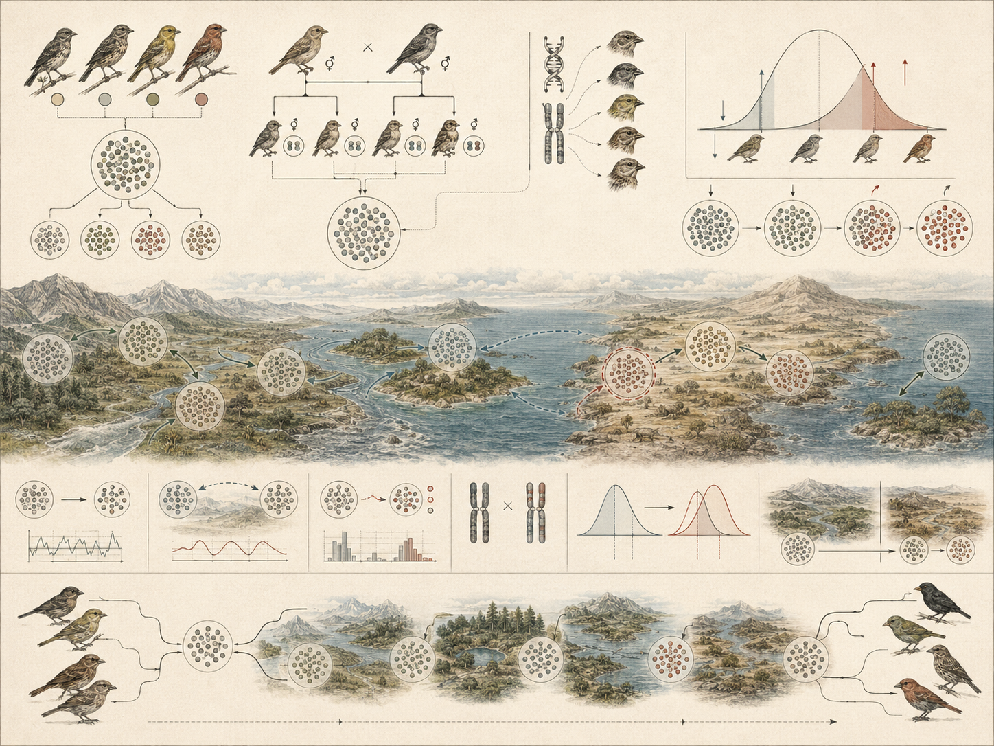
The article develops population genetics and the mathematics of inheritance across heredity, population structure, allele frequency, genotype frequency, Hardy-Weinberg expectations, selection, drift, mutation, migration, recombination, heterozygosity, effective population size, fixation, loss, inbreeding, bottlenecks, gene flow, conservation genetics, pathogen evolution, genomic inference, and computational biology.
The article also extends population genetics into quantitative and computational analysis through Hardy-Weinberg expectations, genotype-frequency calculation, expected heterozygosity, genotype-specific selection, bidirectional mutation, migration, Wright-Fisher drift, fixation and loss statistics, multi-population \(F_{ST}\)-style structure, bottleneck screening, genotype-matrix processing, migration-selection balance, R workflows, Python workflows, SQL provenance structures, and a linked full-stack GitHub repository containing Python, R, Julia, Fortran, Rust, Go, C, C++, SQL, notebooks, data files, validation notes, and reproducibility documentation.
What population genetics is
Population genetics is the study of how allele and genotype frequencies change through time in populations under the influence of processes such as natural selection, genetic drift, mutation, migration, recombination, nonrandom mating, and reproduction. It is foundational because it makes inheritance mathematically explicit at the level where evolution actually occurs: not in isolated individuals, but in populations distributed across generations. Classical genetics can explain how traits are transmitted within families or experimental crosses. Population genetics explains how entire populations shift, persist, diverge, lose variation, or retain adaptive potential.
This matters because the population is the entity whose genetic composition changes historically. The individual organism is the bearer of a genotype, but selection, drift, migration, and mutation alter the relative abundance of variants in the population. They do not transform one adult organism into another type. They change which lineages contribute more genetic copies to the future. Population genetics therefore turns inheritance into a historical science of frequencies, expectations, probabilities, and generational change.
It is also one of biology’s most important integrative frameworks. A field biologist tracking gene flow among fragmented habitats, a clinical researcher interpreting variant frequencies, a microbial ecologist studying resistance evolution, a conservation geneticist evaluating inbreeding, and a crop scientist managing breeding populations all rely, whether explicitly or implicitly, on population-genetic reasoning. The field is mathematical, but its questions are ecological, historical, medical, agricultural, and biological through and through.
Population genetics therefore sits at the center of modern evolutionary biology. It gives scientists a way to ask whether populations are stable, diverging, adapting, drifting, bottlenecked, admixed, inbred, structured, or losing diversity. It is one of the main reasons inheritance can be studied not only as a family-level pattern, but as a population-level process shaping the future of living systems.
From individual inheritance to population change
One of population genetics’ main achievements is showing that inheritance must often be studied at more than the pedigree level. A Mendelian cross tells us how alleles may combine in offspring, but population genetics asks what happens when those combinations are repeated across many individuals and many generations. The key question becomes not simply what offspring one cross can produce, but how common different alleles and genotypes become in a population through time.
This shift in scale is what makes population genetics central to evolutionary biology. It clarifies why evolution is often defined as change in allele frequencies within a population. Selection, drift, migration, mutation, and recombination all operate by altering the relative abundance, arrangement, and transmission of variants in the population. Even when those forces are expressed through individual survival or reproduction, their consequences are measured at the level of frequency change.
Population genetics therefore converts heredity into a science of repeated structure. It asks how inheritance behaves when demographic size, mating pattern, migration, selection intensity, mutation rate, recombination, spatial structure, stochastic sampling, and environmental variation all matter. That is why it is indispensable wherever biology needs to move from individual cases to historical population processes.
This population-level perspective also changes how biological risk is understood. A single organism may appear healthy, but its population may be genetically depleted. A species may remain locally visible, while isolated subpopulations lose heterozygosity. A pathogen may appear controlled, while rare resistant alleles are rising. A restored plant population may establish briefly, while lacking enough genetic diversity for long-term adaptation. Population genetics makes these hidden dynamics visible.
Alleles, genotypes, and frequency
The basic language of population genetics begins with alleles and genotypes. Alleles are alternative forms of a gene or locus, while genotypes are the combinations of alleles carried by individuals. Population genetics then asks how common each allele and genotype is. Allele frequency describes the proportion of all copies of a gene that are of a given type. Genotype frequency describes the proportion of individuals with a given genotype. These concepts are simple, but they are the mathematical foundation on which the rest of the field is built.
This matters because population change is most clearly expressed through frequency change. If one allele rises from rarity to commonness, if heterozygotes become less common than expected, or if allele frequencies differ sharply among populations, the population’s genetic structure has changed. Frequency language therefore lets biology measure inheritance at scale instead of describing it impressionistically.
Once alleles and genotypes are expressed as frequencies, biology can ask sharper questions. Is a population near equilibrium? Is selection acting? Is drift strong? Are migrants entering? Is there evidence of nonrandom mating or population subdivision? Are some loci behaving differently from others? Has a bottleneck reduced genetic diversity? Are resistance alleles spreading? Population genetics is the framework through which such questions become mathematically tractable.
Frequency thinking is also important because rare variants, common variants, heterozygotes, and structured distributions have different biological meanings. A rare allele may be newly arisen, deleterious, locally adaptive, introduced by migration, or rising under selection. A common allele may be ancient, neutral, selected, or simply retained by demographic history. A deficit of heterozygotes may suggest inbreeding, hidden population structure, or technical error. Population genetics does not make these interpretations automatic, but it provides the formal language needed to investigate them.
The Hardy-Weinberg principle
The Hardy-Weinberg principle is one of the field’s most important results because it provides a null model for genetic stability in a population. For a locus with two alleles of frequencies \(p\) and \(q\), where \(p+q=1\), expected genotype frequencies under idealized equilibrium assumptions are \(p^2\), \(2pq\), and \(q^2\). This principle matters not because real populations perfectly satisfy all its assumptions, but because departures from it are informative.
If observed genotype frequencies differ substantially from Hardy-Weinberg expectations, that may suggest selection, nonrandom mating, population structure, inbreeding, migration, mutation, genotyping error, sampling effects, or life-stage sampling bias. In that sense, Hardy-Weinberg equilibrium is less a claim about how all populations truly are than a baseline against which real populations can be interpreted. It is one of biology’s great examples of an idealized mathematical model becoming useful precisely because reality departs from it in meaningful ways.
The principle is therefore both elegant and practical. It turns heredity into a statistical expectation and allows biology to detect when real populations are being shaped by evolutionary or demographic forces. It remains central to teaching, inference, genomics quality control, association studies, conservation genetics, and population-level reasoning across fields.
Hardy-Weinberg reasoning also prevents a common mistake: assuming that genetic inheritance automatically causes allele frequencies to change. Under the idealized assumptions, allele frequencies remain stable from one generation to the next, even though genotype frequencies are reshuffled through reproduction. Evolutionary change requires forces that alter allele frequencies or structure. This is why the principle is so powerful. It separates inheritance alone from evolutionary force.
Evolution as change in allele frequency
One of the clearest population-genetic definitions of evolution is change in allele frequencies over time. This definition is powerful because it captures evolutionary change in a population-level, measurable way. Evolution is not primarily a claim that organisms improve, become more complex, or progress toward a single goal. It is a claim that populations change genetically through time.
This matters because allele-frequency change can be adaptive, neutral, constrained, or even maladaptive under new environmental conditions. Selection may increase advantageous variants. Drift may fix or lose variants by chance. Migration may shift frequencies by moving alleles among populations. Mutation may introduce new variants that later become relevant to adaptation or disease. Recombination may reshape associations among loci, creating new combinations of existing variation. Population genetics provides the language for describing these changes precisely rather than metaphorically.
In that sense, the field translates the grand narrative of evolution into the mathematics of inherited frequencies. It makes historical change measurable, comparable, and testable across systems as different as marine metapopulations, pathogen lineages, crop breeding populations, endangered wildlife, invasive species, human genomic datasets, and microbial communities.
This definition also clarifies why evolution can happen without visible morphological change and why visible phenotypic change does not always imply genetic evolution. A population can change genetically at loci invisible to casual observation. Conversely, organisms can change appearance through plasticity without allele frequencies shifting. Population genetics helps distinguish inherited change from environmental response, which is essential in ecology, conservation, medicine, agriculture, and environmental monitoring.
Selection, drift, mutation, migration, and recombination
Population genetics is especially powerful because it does not reduce evolution to one mechanism. Selection sorts variants nonrandomly by reproductive success. Drift changes frequencies by chance, especially in finite populations. Mutation introduces new sequence differences. Migration moves alleles among populations. Recombination reshuffles existing variation into new combinations. Reproduction itself determines how these forces are transmitted across generations.
This matters because population change is often the result of interacting forces rather than one isolated cause. A rare allele may spread because it is advantageous, because migrants introduced it, because drift raised it by chance in a small population, or because those processes interacted. Likewise, standing genetic variation may be preserved or lost depending on demographic size, mating structure, environmental variability, and temporal fluctuation in selective pressure.
It also means the mathematics of inheritance is inseparable from ecology and demography. The same allele can behave differently in large and small populations, connected and isolated populations, stable and rapidly changing environments, or host-associated and free-living microbial communities. Population genetics gives biology a way to separate, compare, and model those possibilities without pretending that real populations are simple.
Recombination deserves special attention because it changes associations among alleles. Selection may favor a combination of variants, but recombination can break that combination apart. Conversely, recombination can bring beneficial variants together. Population genetics therefore examines not only allele frequency at individual loci, but also linkage, haplotypes, and associations across genomes. In the genomic era, this has become especially important for understanding adaptation, disease association, demographic history, and selection scans.
Population structure, inbreeding, and effective population size
Real populations are rarely perfectly mixed. They are often structured by geography, habitat, social behavior, reproductive timing, host association, dispersal limits, environmental gradients, barriers, currents, watersheds, breeding systems, and historical demography. Population structure matters because allele frequencies may differ among subpopulations even when those subpopulations are part of the same broader species or metapopulation.
This is important because hidden structure can produce misleading conclusions. A combined sample may appear to deviate from Hardy-Weinberg expectations not because individuals are mating nonrandomly within each subpopulation, but because the sample mixes subpopulations with different allele frequencies. This is often called a Wahlund-type effect. In practical terms, ignoring structure can distort association studies, conservation units, ancestry inference, and ecological interpretation.
Inbreeding is another central concern because it increases the probability that individuals inherit identical copies of alleles from shared ancestry. Inbreeding can reduce heterozygosity, expose recessive deleterious alleles, and contribute to inbreeding depression in small or isolated populations. It is especially important in conservation biology, captive breeding, restoration, endangered species management, and small population ecology.
Effective population size, often denoted \(N_e\), is also crucial. It is not simply the number of organisms present. It is a measure of how many individuals effectively contribute genetic copies to future generations. Unequal sex ratios, variance in reproductive success, fluctuating population size, overlapping generations, and bottlenecks can make effective population size much smaller than census size. Because drift depends strongly on effective size, a population that appears numerically large may still lose genetic diversity rapidly if only a small fraction of individuals contribute genetically to future generations.
Population genetics and the logic of inheritance
Population genetics matters because it extends the logic of inheritance beyond family resemblance. Mendelian genetics explains how alleles segregate and assort. Population genetics explains how those alleles behave in aggregate when reproduction, variation, and evolutionary forces are repeated across generations. This is why it occupies such a crucial place between classical genetics and evolutionary theory.
The field helps biology answer questions that pure pedigree analysis cannot answer well on its own. Why does a recessive allele remain in a population? Why does heterozygosity decline in some contexts? Why do small populations lose variation quickly? Why do neighboring populations diverge? Why do some loci show departures from equilibrium while others do not? Why can gene flow homogenize some parts of a genome while selection differentiates others? Population genetics turns these into formal questions rather than loose descriptive puzzles.
In that sense, the mathematics of inheritance is not an optional add-on to biology. It is one of the major ways biology understands how heredity becomes history, how variation becomes structure, and how populations remain dynamic through time.
This logic also supports biological humility. A single gene, trait, or population snapshot rarely tells the whole story. Population genetics asks how frequencies change, how structure is distributed, how chance interacts with selection, and how demographic history shapes what remains visible. It therefore helps biology move from isolated facts toward historical inference.
Population genetics in ecology, conservation, and sustainability
Population genetics is deeply relevant to ecology and sustainability-adjacent biology because ecological resilience, adaptation, and persistence all depend partly on how variation is distributed within and among populations. Conservation concerns such as inbreeding, fragmentation, bottlenecks, isolation, adaptive potential, and genetic rescue are population-genetic concerns at their core.
This matters because environmental disruption often changes not only abundance but also genetic composition. Small isolated populations may lose diversity through drift. Fragmented populations may experience reduced gene flow. Rapid environmental change may outpace adaptive shifts. Strong directional selection may preserve persistence in the short term while reducing diversity in the long term. Population genetics helps make those risks legible in long-horizon ecological terms.
For sustainability-oriented biology, this makes the field indispensable. Populations do not persist only by remaining numerically present. They also need enough inherited diversity and demographic continuity to remain evolutionarily viable. This is a population-genetic way of describing resilience, restoration potential, local adaptation, and long-term ecological integrity.
Restoration ecology especially needs this framework. A restoration project may introduce organisms to a site, but whether those organisms establish, reproduce, and persist depends partly on genetic diversity, local adaptation, inbreeding risk, source-population choice, gene flow, and future environmental change. Population genetics helps restoration move beyond simple reintroduction toward long-term evolutionary viability.
Marine, freshwater, soil, plant, and microbial relevance
Marine biology is deeply population-genetic because marine organisms often occupy large but structured populations spread across currents, temperature gradients, oxygen regimes, salinity fronts, depth zones, larval dispersal networks, and fragmented habitats. Gene flow, local adaptation, drift, and selection can interact in complex ways in fish, corals, plankton, algae, marine invertebrates, and marine microbes. A population-genetic framework is therefore essential to understanding persistence and divergence in oceans under climate stress, acidification, exploitation, hypoxia, and habitat disruption.
Freshwater systems show similar issues where river structure, basin isolation, wetlands, pollution, eutrophication, hydrologic fragmentation, and local adaptation shape population subdivision and adaptive challenge. Freshwater organisms often occupy naturally or artificially isolated systems, making drift, founder effects, restricted gene flow, and local adaptation especially important. Conservation in freshwater systems often requires understanding not only species presence, but genetic connectivity across watersheds and habitats.
Soil biology and microbiology are equally relevant because microbial communities are often immense, dynamic, and evolutionarily responsive, with drift and selection acting on variation under shifting nutrient, moisture, pH, oxygen, and redox conditions. Microbial populations may exchange genes horizontally, experience strong selection, and shift rapidly under disturbance. Population thinking therefore extends far beyond charismatic vertebrates.
Plant science, agroecology, forestry, and restoration ecology also depend on population genetics through seed systems, breeding populations, local adaptation, disease resistance, pollen flow, hybridization, inbreeding, and long-term demographic resilience. The mathematics of inheritance becomes directly practical in these fields whenever genetic composition shapes persistence or response to environmental stress.
Medical, biomedical, and disease ecology relevance
Population genetics matters to medicine and biomedicine because allele frequencies, genotype distributions, and departures from equilibrium can all matter for disease risk, carrier frequency, variant interpretation, pharmacogenomics, and the genetics of populations under treatment or pathogen pressure. Hardy-Weinberg methods remain widely used in human genetics and genomic quality control because they offer a first-pass way to detect unexpected structure, inbreeding, technical problems, or sampling issues.
It also matters because pathogens evolve as populations. Resistance, virulence, host adaptation, immune escape, drug tolerance, and strain replacement are population-level processes shaped by mutation, drift, selection, recombination, and migration. Disease ecology extends this further by linking host and pathogen population structure to transmission and adaptation across environments. A resistant pathogen lineage spreading through hospitals, farms, aquaculture systems, or aquatic environments is a population-genetic event as much as an epidemiological one.
Population genetics therefore helps connect inheritance mathematics to clinical and epidemiological consequence. It is one of the clearest places where abstract frequency models become biologically, medically, and socially consequential.
The same logic applies to cancer, where cell lineages within a tumor may vary, compete, drift, and be selected under therapy. Although tumor evolution is not identical to organismal population genetics, the concepts of clonal frequency, selection, bottleneck, resistance, drift, and lineage expansion are population-genetic in spirit. Medicine increasingly needs this kind of frequency-based thinking because disease is often dynamic rather than static.
Bioinformatics, genomics, and computational relevance
Population genetics has become even more important in the genomic era because large-scale datasets make it possible to estimate allele frequencies, test Hardy-Weinberg expectations, infer structure, scan genomes for selection, estimate effective population size, compare variation across many loci, detect admixture, and reconstruct demographic history. What began as algebra over one or two loci has become a computational science of genotype matrices, sequence variants, simulations, and statistical inference.
Bioinformatics is essential here because the field now depends on large genotype datasets, variant filtering, missing-data handling, resampling, likelihood-based inference, coalescent reasoning, reproducible analysis pipelines, and careful provenance. Yet the conceptual core remains the same: frequencies, expectations, probabilities, and change through time. Modern genomics has not displaced classical population genetics. It has greatly expanded its resolution and practical importance.
This makes population genetics one of the strongest bridges between classical mathematical biology and contemporary data-intensive life science. It is one of the main areas where biological interpretation and computational rigor must remain tightly connected.
Computational population genetics also requires caution. A genotype matrix is shaped by sequencing depth, variant calling, filtering thresholds, reference genomes, missing data, sample structure, batch effects, and sampling design. A statistically impressive result may still be biologically misleading if population structure, relatedness, or demographic history is ignored. Strong population-genetic analysis therefore requires reproducibility, metadata, provenance, and ecological interpretation alongside computation.
Quantitative population genetics: mathematics, R, and Python
Population genetics is inherently mathematical because its core questions concern proportions, expectations, probabilities, stochastic sampling, and generational change. The point of modeling is not to decorate heredity with equations, but to make evolutionary process explicit enough to be compared, simulated, and tested.
For a two-allele locus, if the frequency of one allele is \(p\) and the other is \(q\), then:
p+q=1
\]
Interpretation: At a biallelic locus, the two allele frequencies sum to one.
Under Hardy-Weinberg equilibrium assumptions, expected genotype frequencies are:
p^2+2pq+q^2=1
\]
Interpretation: Expected genotype frequencies follow from allele frequencies under idealized assumptions.
where \(p^2\) is the expected frequency of one homozygote, \(2pq\) the heterozygote, and \(q^2\) the other homozygote.
One of the most useful summary measures of genetic variation at a two-allele locus is expected heterozygosity:
H_e=2pq
\]
Interpretation: Expected heterozygosity summarizes the expected frequency of heterozygotes at a biallelic locus.
This matters because many ecological and conservation questions concern how much variation remains available within populations rather than only which allele is currently common.
If genotype fitnesses are \(W_{AA}\), \(W_{Aa}\), and \(W_{aa}\), then mean population fitness is:
\bar{W}=p^2W_{AA}+2pqW_{Aa}+q^2W_{aa}
\]
Interpretation: Mean population fitness is the genotype-frequency-weighted average of genotype-specific fitness values.
The next-generation allele frequency of \(A\) can be written as:
p’=\frac{p^2W_{AA}+pqW_{Aa}}{\bar{W}}
\]
Interpretation: Genotype-specific selection changes allele frequency through differential reproductive contribution.
This is useful because it formalizes how genotype-specific fitness differences change allele frequencies across generations.
If allele \(A\) mutates to \(a\) at rate \(\mu\) and the reverse occurs at rate \(\nu\), then a simple mutation update is:
p’=p(1-\mu)+q\nu
\]
Interpretation: Mutation shifts allele frequency by removing copies through forward mutation and adding copies through reverse mutation.
If migrants enter at fraction \(m\) from a source population with allele frequency \(p_m\), then the migration update is:
p’=(1-m)p+mp_m
\]
Interpretation: Migration shifts the local allele frequency toward the allele frequency in the migrant source population.
These matter because real populations are rarely closed and mutation-free. New alleles appear, and populations exchange genetic material through movement.
In a diploid Wright-Fisher population of size \(N\), the number of copies of allele \(A\) in the next generation can be treated as a random sample:
X_{t+1}\sim\mathrm{Binomial}(2N,p_t)
\]
Interpretation: The next-generation allele count is sampled from \(2N\) allele copies with probability \(p_t\).
so that:
p_{t+1}=\frac{X_{t+1}}{2N}
\]
Interpretation: The next allele frequency is the sampled allele count divided by the total number of allele copies.
This is useful because it makes explicit that even without selection, allele frequencies fluctuate through finite sampling.
A common way to summarize population structure is through the relation between total heterozygosity and within-population heterozygosity:
F_{ST}=\frac{H_T-H_S}{H_T}
\]
Interpretation: \(F_{ST}\)-style summaries estimate how much genetic variation is partitioned among populations relative to total variation.
where \(H_T\) is expected heterozygosity after pooling populations and \(H_S\) is mean expected heterozygosity within populations. This is useful because population subdivision, restricted gene flow, drift, local adaptation, and bottlenecks can make populations genetically differentiated even when they belong to the same broader species.
A simple inbreeding relation can be expressed as:
H_t=H_0\left(1-\frac{1}{2N_e}\right)^t
\]
Interpretation: Expected heterozygosity declines over time under drift, with the rate depending on effective population size.
This is useful because it shows why small effective population size accelerates loss of genetic variation.
Variables, units, and population-genetic interpretation
Quantitative population genetics depends on variables that connect allele frequencies, genotype frequencies, heterozygosity, selection, mutation, migration, drift, structure, inbreeding, and biological interpretation. The table below summarizes several central quantities.
| Symbol or Term | Meaning | Typical Unit or Scale | Population-Genetic Interpretation |
|---|---|---|---|
| \(p, q\) | Allele frequencies | fraction from 0 to 1 | Relative frequency of two alleles in a population or sample |
| \(p^2, 2pq, q^2\) | Expected genotype frequencies | frequency or probability | Hardy-Weinberg baseline genotype expectations |
| \(H_e\) | Expected heterozygosity | fraction from 0 to 1 | Compact measure of genetic diversity at a biallelic locus |
| \(W_{AA}, W_{Aa}, W_{aa}\) | Genotype-specific fitnesses | relative fitness scale | Reproductive contribution of each genotype relative to alternatives |
| \(\bar{W}\) | Mean population fitness | relative fitness | Genotype-frequency-weighted average fitness |
| \(p’\) | Updated allele frequency | fraction from 0 to 1 | Allele frequency after selection, mutation, migration, or another update |
| \(\mu\) | Forward mutation rate | per generation or replication cycle | Rate at which allele \(A\) changes into allele \(a\) |
| \(\nu\) | Reverse mutation rate | per generation or replication cycle | Rate at which allele \(a\) changes into allele \(A\) |
| \(m\) | Migration fraction | fraction from 0 to 1 | Share of local genetic contribution coming from migrants |
| \(p_m\) | Migrant-source allele frequency | fraction from 0 to 1 | Allele frequency in the source population contributing migrants |
| \(N\) | Diploid population size in a simple model | individuals | Population size determining sampling strength in Wright-Fisher drift |
| \(N_e\) | Effective population size | effective breeding individuals | Population size relevant to drift and genetic diversity loss |
| \(X_{t+1}\) | Sampled allele count | count from 0 to \(2N\) | Number of allele copies sampled into the next generation |
| \(p_t, p_{t+1}\) | Allele frequency at generation \(t\) and \(t+1\) | fraction from 0 to 1 | Allele-frequency trajectory through time |
| \(H_T\) | Total expected heterozygosity | fraction from 0 to 1 | Diversity expected after pooling subpopulations |
| \(H_S\) | Mean within-population heterozygosity | fraction from 0 to 1 | Average diversity within subpopulations |
| \(F_{ST}\) | Population-differentiation statistic | dimensionless fraction-like statistic | Proportion of variation partitioned among populations under the model |
| \(H_t\) | Heterozygosity at time \(t\) | fraction from 0 to 1 | Expected diversity remaining after drift over time |
| Fixation | Allele reaches frequency 1 | state or probability | Allele becomes the only allele at the locus in the population |
| Loss | Allele reaches frequency 0 | state or probability | Allele disappears from the population |
The table shows why population-genetic quantities require context. An allele frequency, genotype expectation, \(F_{ST}\)-style statistic, effective population size, or heterozygosity estimate becomes biologically meaningful only when linked to sampling design, population structure, reproductive system, organism, timescale, environmental condition, and analytical pipeline.
Worked example: Hardy-Weinberg, selection, drift, and structure
Suppose allele \(A\) has frequency \(p=0.7\). Then allele \(a\) has frequency:
q=1-p=1-0.7=0.3
\]
Interpretation: At a two-allele locus, the second allele frequency follows once the first is known.
Expected genotype frequencies are:
AA=p^2=(0.7)^2=0.49
\]
Interpretation: The expected \(AA\) frequency is 0.49 under Hardy-Weinberg assumptions.
Aa=2pq=2(0.7)(0.3)=0.42
\]
Interpretation: The expected heterozygote frequency is 0.42.
aa=q^2=(0.3)^2=0.09
\]
Interpretation: The expected \(aa\) frequency is 0.09.
Expected heterozygosity is:
H_e=2pq=2(0.7)(0.3)=0.42
\]
Interpretation: The expected heterozygosity at this locus is 0.42.
This gives a baseline against which observed population data can be compared.
Now suppose genotype fitnesses are \(W_{AA}=1.10\), \(W_{Aa}=1.02\), and \(W_{aa}=1.00\). Mean fitness is:
\bar{W}=0.49(1.10)+0.42(1.02)+0.09(1.00)=1.0574
\]
Interpretation: Mean fitness is the genotype-weighted average of relative fitness.
The next-generation frequency of allele \(A\) after selection is:
p’=\frac{0.49(1.10)+(0.7)(0.3)(1.02)}{1.0574}\approx0.7116
\]
Interpretation: Selection increases allele \(A\) from 0.7000 to approximately 0.7116 under this model.
This shows how genotype-specific fitness differences translate into allele-frequency change.
For drift, suppose a diploid population has \(N=50\), so there are \(2N=100\) allele copies. If \(p_t=0.7\), the expected number of \(A\) copies is:
E[X_{t+1}]=2Np_t=100(0.7)=70
\]
Interpretation: The expected next-generation allele-copy count is 70, but the realized count can differ by chance.
This is useful because drift is not a deterministic force pushing in one direction. It is stochastic sampling, and its effects are stronger when effective population size is small.
For population structure, suppose total heterozygosity after pooling populations is \(H_T=0.48\), while mean within-population heterozygosity is \(H_S=0.36\). Then:
F_{ST}=\frac{H_T-H_S}{H_T}=\frac{0.48-0.36}{0.48}=0.25
\]
Interpretation: Under this simplified calculation, 25 percent of the modeled variation is partitioned among populations.
This is useful because it shows how population subdivision can be summarized quantitatively, while still requiring careful biological interpretation.
Computational modeling
Computational modeling helps make population genetics explicit because population-genetic reasoning is dynamic, stochastic, structured, and data-intensive. Hardy-Weinberg models provide baselines. Selection models update allele frequencies through genotype-specific reproductive success. Mutation and migration models add new variants or move variants among populations. Wright-Fisher simulations show stochastic drift across replicate populations. \(F_{ST}\)-style summaries represent structured differentiation. Genotype-matrix workflows turn raw coded genotype data into allele frequencies and equilibrium screens. Migration-selection models help analyze local adaptation under gene flow.
The selected examples below focus on compact, reusable workflows: Hardy-Weinberg expectations, genotype-specific selection, bidirectional mutation, migration, Wright-Fisher drift, heterozygosity trajectories, fixation and loss statistics, multi-population \(F_{ST}\)-style structure, bottleneck screening, genotype-matrix processing, and migration-selection balance. The GitHub repository extends the same logic into richer workflows for SQL provenance, reproducible data files, validation notes, notebooks, simulation scenarios, and multi-language scientific-computing examples.
The purpose is not to reduce inheritance to code. The purpose is to make population-genetic reasoning inspectable. A population-genetic claim becomes stronger when allele counts, genotype matrices, sample metadata, population definitions, filtering rules, assumptions, simulation parameters, and analytical code are documented together.
R workflow: selection, mutation, migration, drift, and population structure
R is useful for population genetics because it supports simulation, statistical summaries, tabular workflows, multi-population analysis, and reproducible reporting. The following workflow simulates a diploid two-allele locus under genotype-specific selection, bidirectional mutation, migration, and optional Wright-Fisher drift; then estimates multi-population \(F_{ST}\)-style structure and bottleneck-like differentiation.
# Population Genetics and the Mathematics of Inheritance Workflow
#
# This workflow demonstrates four quantitative population-genetics tasks:
#
#   1. Simulate a two-allele diploid locus under selection, mutation,
#      migration, and optional Wright-Fisher drift.
#   2. Compare multiple evolutionary scenarios.
#   3. Estimate expected heterozygosity through time.
#   4. Simulate multi-population structure and FST-style differentiation.
#
# These examples can be adapted for evolutionary biology, conservation
# genetics, restoration ecology, pathogen evolution, crop breeding,
# marine and freshwater population structure, and computational genomics.

library(dplyr)
library(tidyr)
library(purrr)
library(tibble)

# ------------------------------------------------------------
# 1. Two-allele population-genetic simulation
# ------------------------------------------------------------

simulate_pg <- function(
  generations = 150,
  p0 = 0.5,
  N = 500,
  W_AA = 1.0,
  W_Aa = 1.0,
  W_aa = 1.0,
  mu = 0.000,
  nu = 0.000,
  m = 0.000,
  p_migrant = 0.5,
  drift = TRUE,
  seed = 123
) {
  set.seed(seed)

  p <- numeric(generations + 1)
  q <- numeric(generations + 1)
  Hexp <- numeric(generations + 1)
  Wbar <- numeric(generations + 1)

  p[1] <- p0
  q[1] <- 1 - p0
  Hexp[1] <- 2 * p0 * (1 - p0)
  Wbar[1] <- NA_real_

  for (t in 1:generations) {
    pt <- p[t]
    qt <- 1 - pt

    f_AA <- pt^2
    f_Aa <- 2 * pt * qt
    f_aa <- qt^2

    wbar <- f_AA * W_AA + f_Aa * W_Aa + f_aa * W_aa

    p_sel <- (
      f_AA * W_AA + 0.5 * f_Aa * W_Aa
    ) / wbar

    q_sel <- 1 - p_sel

    p_mut <- p_sel * (1 - mu) + q_sel * nu

    p_mig <- (1 - m) * p_mut + m * p_migrant

    if (drift) {
      count_A <- rbinom(1, size = 2 * N, prob = p_mig)
      p_next <- count_A / (2 * N)
    } else {
      p_next <- p_mig
    }

    p[t + 1] <- p_next
    q[t + 1] <- 1 - p_next
    Hexp[t + 1] <- 2 * p_next * (1 - p_next)
    Wbar[t + 1] <- wbar
  }

  tibble(
    generation = 0:generations,
    p = p,
    q = q,
    expected_heterozygosity = Hexp,
    mean_fitness = Wbar
  )
}

scenarios <- tibble(
  scenario = c(
    "neutral_large_population",
    "selection_for_A",
    "migration_balance",
    "mutation_selection_balance"
  ),
  p0 = c(0.50, 0.20, 0.90, 0.99),
  N = c(5000, 1000, 1000, 3000),
  W_AA = c(1.00, 1.15, 1.00, 1.00),
  W_Aa = c(1.00, 1.08, 1.00, 0.98),
  W_aa = c(1.00, 1.00, 1.00, 0.92),
  mu = c(0.0000, 0.0000, 0.0000, 0.0015),
  nu = c(0.0000, 0.0000, 0.0000, 0.0001),
  m = c(0.000, 0.000, 0.040, 0.000),
  p_migrant = c(0.50, 0.50, 0.15, 0.50),
  drift = c(TRUE, TRUE, TRUE, FALSE)
)

results <- scenarios %>%
  mutate(
    sim = pmap(
      list(p0, N, W_AA, W_Aa, W_aa, mu, nu, m, p_migrant, drift),
      function(p0, N, W_AA, W_Aa, W_aa, mu, nu, m, p_migrant, drift) {
        simulate_pg(
          generations = 180,
          p0 = p0,
          N = N,
          W_AA = W_AA,
          W_Aa = W_Aa,
          W_aa = W_aa,
          mu = mu,
          nu = nu,
          m = m,
          p_migrant = p_migrant,
          drift = drift,
          seed = 123
        )
      }
    )
  ) %>%
  select(scenario, sim) %>%
  unnest(sim)

summary_tbl <- results %>%
  group_by(scenario) %>%
  summarise(
    initial_p = first(p),
    final_p = last(p),
    final_H = last(expected_heterozygosity),
    final_mean_fitness = last(mean_fitness),
    .groups = "drop"
  )

# ------------------------------------------------------------
# 2. Multi-population FST-style structure
# ------------------------------------------------------------

simulate_structure <- function(pops = 4, loci = 250, bottleneck_pop = 3) {
  ancestral_p <- runif(loci, 0.1, 0.9)

  pop_freqs <- map_dfc(1:pops, function(i) {
    drift_scale <- if (i == bottleneck_pop) 35 else 120
    counts <- rbinom(loci, size = drift_scale, prob = ancestral_p)

    tibble(!!paste0("pop", i) := counts / drift_scale)
  })

  allele_freqs <- bind_cols(tibble(locus = 1:loci), pop_freqs)

  long_df <- allele_freqs %>%
    pivot_longer(
      cols = -locus,
      names_to = "population",
      values_to = "p"
    )

  fst_summary <- long_df %>%
    group_by(locus) %>%
    summarise(
      pbar = mean(p),
      HS = mean(2 * p * (1 - p)),
      HT = 2 * pbar * (1 - pbar),
      fst = ifelse(HT > 0, (HT - HS) / HT, 0),
      .groups = "drop"
    )

  list(
    allele_freqs = allele_freqs,
    fst_summary = fst_summary,
    genome_wide_mean_fst = mean(fst_summary$fst)
  )
}

set.seed(42)
structure_results <- simulate_structure()

top_structured_loci <- structure_results$fst_summary %>%
  arrange(desc(fst)) %>%
  slice_head(n = 20)

# ------------------------------------------------------------
# 3. Print compact outputs
# ------------------------------------------------------------

print(summary_tbl %>% mutate(across(where(is.numeric), round, 4)))

print(
  results %>%
    filter(generation %in% c(0, 20, 50, 100, 150, 180)) %>%
    mutate(across(where(is.numeric), round, 4))
)

print(structure_results$allele_freqs %>% slice_head(n = 10))
print(top_structured_loci %>% mutate(across(where(is.numeric), round, 4)))

cat(
  "Genome-wide mean FST:",
  round(structure_results$genome_wide_mean_fst, 4),
  "\n"
)
This R workflow is useful because it moves beyond static Hardy-Weinberg expectations and shows how different mechanisms interact across time. It provides a practical scaffold for evolutionary reasoning about allele trajectories, heterozygosity loss, selection response, mutation-selection balance, migration-driven frequency change, population differentiation, and bottleneck-like structure.
Python workflow: Wright-Fisher replicates, genotype matrices, Hardy-Weinberg screening, and migration-selection balance
Python is useful for population genetics because it supports stochastic simulation, genotype-matrix processing, numerical analysis, time-series workflows, and reproducible computation. The following workflow simulates Wright-Fisher allele-frequency trajectories with selection, estimates fixation and loss statistics, processes coded genotype matrices for Hardy-Weinberg screening, and models migration-selection balance across two populations.
"""
Population Genetics and the Mathematics of Inheritance Workflow

This workflow demonstrates four quantitative population-genetics tasks:

1. Simulate Wright-Fisher allele-frequency trajectories with selection.
2. Estimate fixation, loss, and heterozygosity statistics across replicates.
3. Process a genotype matrix to estimate allele frequencies and
   Hardy-Weinberg expected counts.
4. Simulate migration-selection balance across two populations.

The examples are compact, but the same structures can be extended to
conservation genetics, disease ecology, population genomics, crop breeding,
marine and freshwater population structure, pathogen evolution, and
computational biology.
"""

from __future__ import annotations

import numpy as np
import pandas as pd


def wright_fisher_replicates(
    generations: int = 250,
    N: int = 150,
    p0: float = 0.25,
    w_AA: float = 1.10,
    w_Aa: float = 1.05,
    w_aa: float = 1.00,
    replicates: int = 300,
    seed: int = 42,
) -> tuple[pd.DataFrame, pd.DataFrame, pd.DataFrame]:
    """
    Simulate Wright-Fisher allele-frequency trajectories with selection.
    """
    rng = np.random.default_rng(seed)

    records = []

    for rep in range(replicates):
        p = p0

        for gen in range(generations + 1):
            records.append(
                {
                    "replicate": rep,
                    "generation": gen,
                    "p": p,
                    "q": 1.0 - p,
                    "heterozygosity": 2.0 * p * (1.0 - p),
                }
            )

            if gen == generations:
                continue

            q = 1.0 - p

            f_AA = p**2
            f_Aa = 2.0 * p * q
            f_aa = q**2

            wbar = f_AA * w_AA + f_Aa * w_Aa + f_aa * w_aa

            p_sel = (
                f_AA * w_AA + 0.5 * f_Aa * w_Aa
            ) / wbar

            count_A = rng.binomial(2 * N, p_sel)
            p = count_A / (2.0 * N)

    df = pd.DataFrame(records)

    summary = (
        df.groupby("generation")
        .agg(
            mean_p=("p", "mean"),
            sd_p=("p", "std"),
            mean_H=("heterozygosity", "mean"),
        )
        .reset_index()
    )

    final_generation = df["generation"].max()
    finals = df[df["generation"] == final_generation].copy()

    final_summary = pd.DataFrame(
        {
            "fixation_probability": [np.mean(finals["p"] == 1.0)],
            "loss_probability": [np.mean(finals["p"] == 0.0)],
            "mean_final_p": [finals["p"].mean()],
            "mean_final_H": [finals["heterozygosity"].mean()],
        }
    )

    return df, summary, final_summary


def summarize_genotype_matrix() -> pd.DataFrame:
    """
    Estimate allele frequency and Hardy-Weinberg expected counts
    from a compact coded genotype matrix.

    Genotype coding:
    0 = aa
    1 = Aa
    2 = AA
    """
    genotype_matrix = pd.DataFrame(
        {
            "locus_1": [2, 1, 1, 0, 2, 1, 2, 0, 1, 2],
            "locus_2": [1, 1, 0, 0, 1, 2, 1, 0, 1, 1],
            "locus_3": [2, 2, 1, 1, 2, 2, 1, 1, 2, 2],
            "locus_4": [0, 0, 0, 1, 0, 1, 0, 0, 1, 0],
        }
    )

    def locus_summary(genotypes: np.ndarray) -> dict[str, float]:
        """
        Estimate allele frequency and Hardy-Weinberg expected counts.
        """
        n = len(genotypes)

        n_AA = int(np.sum(genotypes == 2))
        n_Aa = int(np.sum(genotypes == 1))
        n_aa = int(np.sum(genotypes == 0))

        p = (2 * n_AA + n_Aa) / (2 * n)
        q = 1.0 - p

        exp_AA = p**2 * n
        exp_Aa = 2.0 * p * q * n
        exp_aa = q**2 * n

        chi2 = (
            ((n_AA - exp_AA) ** 2 / exp_AA) if exp_AA > 0 else 0.0
        ) + (
            ((n_Aa - exp_Aa) ** 2 / exp_Aa) if exp_Aa > 0 else 0.0
        ) + (
            ((n_aa - exp_aa) ** 2 / exp_aa) if exp_aa > 0 else 0.0
        )

        return {
            "n": n,
            "p": p,
            "q": q,
            "obs_AA": n_AA,
            "obs_Aa": n_Aa,
            "obs_aa": n_aa,
            "exp_AA": exp_AA,
            "exp_Aa": exp_Aa,
            "exp_aa": exp_aa,
            "expected_heterozygosity": 2.0 * p * q,
            "chi2_HW_screen": chi2,
        }

    rows = []

    for locus in genotype_matrix.columns:
        res = locus_summary(genotype_matrix[locus].values)
        res["locus"] = locus
        rows.append(res)

    return pd.DataFrame(rows)


def migration_selection_balance(
    generations: int = 150,
    p1_0: float = 0.8,
    p2_0: float = 0.2,
    m12: float = 0.03,
    m21: float = 0.03,
    s1: float = 0.08,
    s2: float = -0.04,
) -> pd.DataFrame:
    """
    Simulate a simple migration-selection balance scenario across two populations.

    This compact example uses a haploid-style selection approximation for clarity.
    """
    records = []

    p1 = p1_0
    p2 = p2_0

    for gen in range(generations + 1):
        records.append(
            {
                "generation": gen,
                "p1": p1,
                "p2": p2,
                "delta_p": abs(p1 - p2),
            }
        )

        if gen == generations:
            continue

        p1_sel = (p1 * (1.0 + s1)) / (p1 * (1.0 + s1) + (1.0 - p1))
        p2_sel = (p2 * (1.0 + s2)) / (p2 * (1.0 + s2) + (1.0 - p2))

        p1_next = (1.0 - m12) * p1_sel + m12 * p2_sel
        p2_next = (1.0 - m21) * p2_sel + m21 * p1_sel

        p1, p2 = p1_next, p2_next

    return pd.DataFrame(records)


def population_structure_screen(seed: int = 11) -> tuple[pd.DataFrame, pd.DataFrame]:
    """
    Simulate multiple populations and calculate FST-style summaries.
    """
    rng = np.random.default_rng(seed)

    loci = 300
    pops = 4

    ancestral_p = rng.uniform(0.10, 0.90, size=loci)

    data = {"locus": np.arange(1, loci + 1)}

    for pop in range(1, pops + 1):
        drift_scale = 35 if pop == 3 else 120
        counts = rng.binomial(drift_scale, ancestral_p)
        data[f"pop{pop}"] = counts / drift_scale

    allele_freqs = pd.DataFrame(data)

    rows = []

    for _, row in allele_freqs.iterrows():
        freqs = np.array([row[f"pop{pop}"] for pop in range(1, pops + 1)])

        pbar = freqs.mean()
        hs = np.mean(2.0 * freqs * (1.0 - freqs))
        ht = 2.0 * pbar * (1.0 - pbar)

        fst = (ht - hs) / ht if ht > 0 else 0.0

        rows.append(
            {
                "locus": row["locus"],
                "pbar": pbar,
                "HS": hs,
                "HT": ht,
                "fst": fst,
            }
        )

    fst_summary = pd.DataFrame(rows)

    return allele_freqs, fst_summary.sort_values("fst", ascending=False)


def main() -> None:
    """
    Run compact population-genetics workflows.
    """
    _, wf_summary, wf_final = wright_fisher_replicates()
    hw_summary = summarize_genotype_matrix()
    migration_df = migration_selection_balance()
    allele_freqs, fst_summary = population_structure_screen()

    print("Wright-Fisher generation summary:")
    print(wf_summary.head(15).round(4).to_string(index=False))
    print(wf_summary.tail(15).round(4).to_string(index=False))
    print(wf_final.round(4).to_string(index=False))

    print("\nGenotype matrix and Hardy-Weinberg screening:")
    print(hw_summary.round(4).to_string(index=False))

    print("\nMigration-selection balance:")
    print(migration_df.head(20).round(4).to_string(index=False))
    print(migration_df.tail(20).round(4).to_string(index=False))

    print("\nAllele frequency matrix:")
    print(allele_freqs.head(10).round(4).to_string(index=False))

    print("\nTop FST-style differentiated loci:")
    print(fst_summary.head(20).round(4).to_string(index=False))

    print(
        "\nGenome-wide mean FST:",
        round(float(fst_summary["fst"].mean()), 4),
    )


if __name__ == "__main__":
    main()
This Python workflow is useful because it mimics practical population-genomic reasoning: taking genotype data, estimating allele frequencies, screening Hardy-Weinberg expectations, simulating selection and drift, modeling migration-selection balance, and summarizing population structure. It provides a compact bridge between classical population genetics and modern computational biology.
GitHub repository
The article body includes compact R and Python examples so the biological and scientific argument remains readable. The full repository expands those examples into a broader computational population-genetics workflow, including Hardy-Weinberg expectations, genotype-frequency calculation, expected heterozygosity, genotype-specific selection, bidirectional mutation, migration, Wright-Fisher drift, fixation and loss statistics, multi-population \(F_{ST}\)-style structure, bottleneck screening, genotype-matrix processing, migration-selection balance, effective-population-size scenarios, SQL provenance structures, reproducible data files, validation notes, and full-stack scientific-computing examples across Python, R, Julia, Fortran, Rust, Go, C, C++, SQL, and notebooks.
Complete Code Repository
The full code distribution for this article, including selected article examples, expanded computational workflows, reproducible data structures, provenance documentation, validation notes, and full-stack scientific-computing scaffolding, is available on GitHub.
Limits, assumptions, and modern population thinking
Population genetics is powerful, but its classic models are built on assumptions that real populations often violate. Hardy-Weinberg equilibrium assumes an idealized situation, and real populations may depart from it because of selection, drift, migration, mutation, nonrandom mating, hidden structure, life-stage sampling bias, genotyping error, relatedness, or sampling variance. This is not a weakness of the field. It is one of its strengths. Population genetics is useful precisely because it provides a baseline from which real complexity can be studied.
Modern population thinking is therefore both mathematical and biological. It depends on formulas, but it also depends on ecology, demography, history, spatial structure, life history, reproductive systems, and careful interpretation. Genome-scale data do not eliminate this need; they intensify it. Large datasets can sharpen inference, but only when models, assumptions, filtering choices, and biological context are handled with discipline.
Models are useful because they clarify assumptions, expose mechanisms, and make comparison possible. But Hardy-Weinberg expectations are not a full population history, \(F_{ST}\) is not a complete account of structure, and a Wright-Fisher simulation is not the whole complexity of real reproduction. Quantitative tools are strongest when they support biological interpretation rather than replacing it.
Biology is strongest here when it treats population genetics not as a closed algebraic game, but as a rigorous framework for reasoning about how inheritance behaves under real conditions of chance, structure, and environmental change.
This caution is especially important in applied contexts. A conservation decision based on one diversity statistic alone may miss adaptive structure. A medical association study may be confounded by ancestry or population subdivision. A pathogen surveillance result may reflect sampling bias rather than true frequency change. Population genetics is powerful because it formalizes uncertainty, but it demands careful interpretation of uncertainty as well.
Why this matters for scientific work
For working scientists, population genetics matters because many biological problems are misread when inheritance is treated only at the individual level. A conservation problem may hinge on loss of heterozygosity rather than simple decline in census abundance. A disease problem may reflect population structure in the pathogen or host rather than one gene alone. A restoration project may fail because reintroduced populations lack adaptive diversity or because source populations were genetically mismatched to local conditions. A crop or forestry problem may depend on gene flow, inbreeding, or resistance evolution.
This means population genetics should often be treated as explanatory infrastructure rather than as a specialized mathematical corner of biology. Ecologists need it to understand adaptation and fragmentation. Conservation biologists need it to reason about bottlenecks, inbreeding, genetic rescue, and viability. Biomedical scientists need it for variant interpretation and disease association. Microbiologists and disease ecologists need it because resistance and virulence evolve in populations. Plant scientists and agroecologists need it because seed systems, breeding, local adaptation, and disease resistance are population processes. Computational biologists need it because frequency change, structure, and inference are central data problems as well as biological realities.
The scientific importance of population genetics lies partly in this breadth. It is one of the principal ways biology explains how inheritance operates under real conditions of time, population structure, ecological pressure, and evolutionary force.
Population genetics is also practically actionable. Allele frequencies can be estimated. Hardy-Weinberg expectations can be screened. Genetic diversity can be monitored. Migration can be modeled. Structure can be summarized. Bottlenecks can be detected. Fixation and loss can be simulated. These tools connect inheritance mathematics to conservation, medicine, agriculture, restoration ecology, disease ecology, marine and freshwater biology, and genomic science.
Conclusion
Population genetics and the mathematics of inheritance show that heredity becomes evolutionarily meaningful when it is studied at the level of populations. Allele frequencies, genotype expectations, equilibrium models, and deviations from those models allow biology to describe how inherited variation is distributed and how it changes through time under the action of selection, drift, mutation, migration, recombination, mating structure, and reproduction.
To understand population genetics is therefore to understand one of the deepest quantitative foundations of biology. It explains how inheritance becomes history, how evolution becomes measurable, and why the persistence of variation matters so much for ecology, conservation, medicine, disease ecology, agriculture, and sustainability-adjacent biology.
Population genetics is thus more than a mathematical subfield. It is one of the principal ways biology explains how populations remain dynamic through time. Modern computational workflows deepen that understanding by making frequency change, heterozygosity, drift, structure, migration, selection, and population-genetic provenance more transparent, reproducible, and scientifically interpretable.
Related articles
- Biology
- Genes, Inheritance, and the Principles of Heredity
- Natural Selection, Adaptation, and Fitness
- Evolution and the History of Life
- Mutation, Variation, and the Sources of Novelty
- Genomics and the Expansion of Biological Knowledge
- Microevolution, Macroevolution, and Deep Time
- Speciation, Diversity, and the Tree of Life
- Biodiversity and the Structure of Living Systems
- Population Dynamics and Ecological Modeling
- Coevolution, Symbiosis, and the Dynamics of Mutual Change
- Ecology and the Interdependence of Life
Further reading
- Charlesworth, B. and Charlesworth, D. (2010) Elements of Evolutionary Genetics. Greenwood Village, CO: Roberts and Company. Bibliographic information available at: https://www.research.ed.ac.uk/en/publications/elements-of-evolutionary-genetics/
- Falconer, D.S. and Mackay, T.F.C. (1996) Introduction to Quantitative Genetics. 4th edn. Harlow: Longman. Bibliographic information available at: https://search.worldcat.org/title/Introduction-to-quantitative-genetics/oclc/34704925
- Gillespie, J.H. (2004) Population Genetics: A Concise Guide. 2nd edn. Baltimore, MD: Johns Hopkins University Press. Publisher information available at: https://www.press.jhu.edu/books/title/3466/population-genetics
- Hartl, D.L. and Clark, A.G. (2007) Principles of Population Genetics. 4th edn. Sunderland, MA: Sinauer Associates. Bibliographic information available at: https://catalog.nlm.nih.gov/discovery/fulldisplay/alma9912910513406676/01NLM_INST:01NLM_INST
- Hedrick, P.W. (2011) Genetics of Populations. 4th edn. Sudbury, MA: Jones & Bartlett. Publisher information available at: https://www.jblearning.com/catalog/productdetails/9780763757373
- Mayo, O. (2008) ‘A century of Hardy-Weinberg equilibrium’, Twin Research and Human Genetics, 11(3), pp. 249–256. Available at: https://doi.org/10.1375/twin.11.3.249
- Nei, M. (1987) Molecular Evolutionary Genetics. New York: Columbia University Press. Bibliographic information available at: https://search.worldcat.org/title/Molecular-evolutionary-genetics/oclc/15017308
- Sork, V.L. (2015) ‘Gene flow and natural selection shape spatial patterns of genes in tree populations: implications for evolutionary processes and applications’, Evolutionary Applications, 9(1), pp. 291–310. Available at: https://doi.org/10.1111/eva.12191
- Wakeley, J. (2008) Coalescent Theory: An Introduction. Greenwood Village, CO: Roberts and Company. Review information available at: https://academic.oup.com/sysbio/article/58/1/162/1673216
- Wright, S. (1931) ‘Evolution in Mendelian populations’, Genetics, 16(2), pp. 97–159. Available at: https://pmc.ncbi.nlm.nih.gov/articles/PMC1201091/
References
- Charlesworth, B. and Charlesworth, D. (2010) Elements of Evolutionary Genetics. Greenwood Village, CO: Roberts and Company. Bibliographic information available at: https://www.research.ed.ac.uk/en/publications/elements-of-evolutionary-genetics/
- Falconer, D.S. and Mackay, T.F.C. (1996) Introduction to Quantitative Genetics. 4th edn. Harlow: Longman. Bibliographic information available at: https://search.worldcat.org/title/Introduction-to-quantitative-genetics/oclc/34704925
- Gillespie, J.H. (2004) Population Genetics: A Concise Guide. 2nd edn. Baltimore, MD: Johns Hopkins University Press. Publisher information available at: https://www.press.jhu.edu/books/title/3466/population-genetics
- Hartl, D.L. and Clark, A.G. (2007) Principles of Population Genetics. 4th edn. Sunderland, MA: Sinauer Associates. Bibliographic information available at: https://catalog.nlm.nih.gov/discovery/fulldisplay/alma9912910513406676/01NLM_INST:01NLM_INST
- Hedrick, P.W. (2011) Genetics of Populations. 4th edn. Sudbury, MA: Jones & Bartlett. Publisher information available at: https://www.jblearning.com/catalog/productdetails/9780763757373
- Mayo, O. (2008) ‘A century of Hardy-Weinberg equilibrium’, Twin Research and Human Genetics, 11(3), pp. 249–256. Available at: https://doi.org/10.1375/twin.11.3.249
- Nei, M. (1987) Molecular Evolutionary Genetics. New York: Columbia University Press. Bibliographic information available at: https://search.worldcat.org/title/Molecular-evolutionary-genetics/oclc/15017308
- Sork, V.L. (2015) ‘Gene flow and natural selection shape spatial patterns of genes in tree populations: implications for evolutionary processes and applications’, Evolutionary Applications, 9(1), pp. 291–310. Available at: https://doi.org/10.1111/eva.12191
- Wakeley, J. (2008) Coalescent Theory: An Introduction. Greenwood Village, CO: Roberts and Company. Review information available at: https://academic.oup.com/sysbio/article/58/1/162/1673216
- Wright, S. (1931) ‘Evolution in Mendelian populations’, Genetics, 16(2), pp. 97–159. Available at: https://pmc.ncbi.nlm.nih.gov/articles/PMC1201091/