
Last Updated May 28, 2026
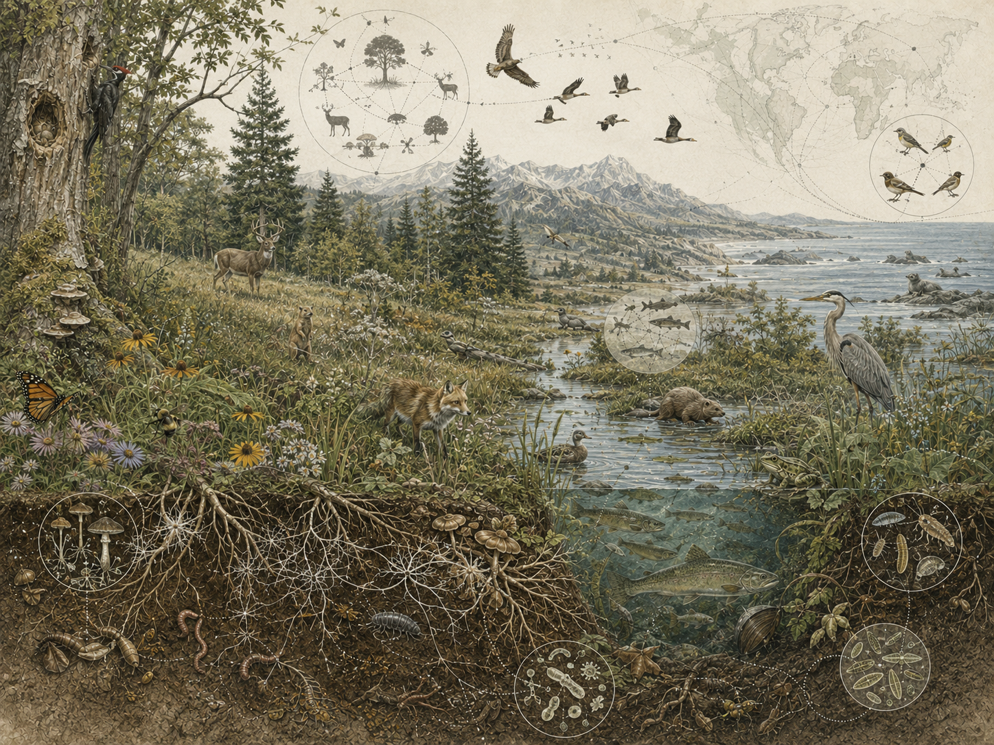
Biodiversity and the structure of living systems examine how life is differentiated, organized, and sustained across genes, populations, species, traits, functional roles, lineages, communities, ecosystems, and biogeographic regions. Biodiversity is not simply a count of species. It is the patterned variety of life across scales, including diversity within species, between species, and among ecosystems. The Convention on Biological Diversity defines biological diversity in exactly those terms, and major global assessments have repeatedly emphasized that biodiversity is fundamental to ecosystem functioning, resilience, adaptation, and the long-term capacity of living systems to persist under change.
Biodiversity is therefore one of biology’s most important structural concepts. It describes how living difference becomes organized into ecological and evolutionary systems. Genetic variation gives populations adaptive capacity. Species diversity shapes community composition and ecological interaction. Functional diversity determines how organisms contribute to production, decomposition, pollination, predation, nutrient cycling, disease regulation, and ecosystem engineering. Phylogenetic diversity preserves evolutionary history. Ecosystem diversity creates the environmental heterogeneity through which populations diverge, communities assemble, and life remains distributed across the biosphere.
Main Library
Publications
Article Map
Biology
Related Topic
Environmental Science
Related Topic
Earth Science
Related Topic
Mathematical Modeling
The article is written for ecologists, marine biologists, freshwater scientists, medical and environmental-health readers, computational biology readers, biodiversity experts, restoration practitioners, conservation planners, and research biologists who need a rigorous account of how living difference is measured, maintained, transformed, and threatened across scales.
The article also extends biodiversity science into quantitative and computational biology through Shannon diversity, Simpson diversity, Hill numbers, beta diversity, ordination, trait-based diversity, functional dispersion, community-weighted means, biodiversity-risk screening, R workflows, Python workflows, SQL provenance structures, and a linked full-stack GitHub repository containing Python, R, Julia, Fortran, Rust, Go, C, C++, SQL, notebooks, data files, and reproducibility documentation.
What biodiversity is
Biodiversity is the variability of life. In the most authoritative policy definition, the Convention on Biological Diversity defines biological diversity as variability among living organisms from all sources, including terrestrial, marine, and other aquatic ecosystems, and the ecological complexes of which they are part; this includes diversity within species, between species, and of ecosystems. That definition remains important because it resists the common mistake of reducing biodiversity to species richness alone. Biodiversity includes genes, populations, species, traits, communities, ecosystems, and ecological complexes. It is therefore a property of the organization of life, not merely a list of named organisms.
This broader definition also explains why biodiversity belongs at the center of biology rather than at its margins. Diversity is how life is distributed across form, function, lineage, interaction, and environment. It is the raw material of adaptation, the substrate of ecological assembly, and one of the principal ways that living systems maintain options under uncertainty. Major assessments have treated biodiversity as foundational to ecosystem functioning and to the continued capacity of ecosystems to support life under pressure.
Biodiversity also connects different biological scales. Genetic diversity influences population resilience, disease resistance, inbreeding risk, and adaptive potential. Species diversity shapes community structure, trophic interactions, and ecosystem functioning. Functional diversity determines whether ecological roles remain available when conditions change. Phylogenetic diversity preserves deep evolutionary history and often captures forms of biological distinctiveness that species counts alone miss. Ecosystem diversity creates the landscape and seascape heterogeneity through which biodiversity is generated and maintained.
For research biologists, this is a crucial point: biodiversity is not a decorative outcome of evolution and ecology. It is one of the main ways the structure of living systems becomes legible.
Why biodiversity is structural, not incidental
Biodiversity is structural because living systems are built through difference. Species occupy different niches, use resources in different ways, vary in life history, respond differently to disturbance, and contribute distinct functional effects to communities and ecosystems. A forest, estuary, grassland, coral reef, wetland, river, agricultural mosaic, or soil system is not simply “alive.” It is organized through layered differences among organisms whose coexistence shapes the structure and behavior of the whole.
This means biodiversity is not an ornamental feature added on top of ecological systems after the fact. It is one of the reasons ecosystems have the form they do. The diversity of producers, consumers, decomposers, symbionts, parasites, pathogens, and engineers determines how matter moves, how energy is transferred, how disturbances are absorbed, and how recovery becomes possible. Communities contain species filling diverse ecological roles, and that diversity can stabilize ecological functioning through time.
The structural importance of biodiversity becomes especially visible when it is lost. A community may retain biomass while losing functional roles. A forest may remain green while losing pollinators, seed dispersers, fungal associates, predators, or specialized understory species. A coral reef may retain physical structure while losing living coral cover and associated fish diversity. A soil system may still support plant growth while losing microbial diversity and nutrient-cycling capacity. Biodiversity loss is therefore not only subtraction from a species list. It can be a reorganization of biological architecture.
The deeper implication is that biodiversity is not external to biological explanation. It is internal to the causal architecture of living systems.
Genetic, species, and ecosystem diversity
The conventional tripartite structure of biodiversity distinguishes genetic diversity, species diversity, and ecosystem diversity. Genetic diversity concerns variation within species and populations. It matters because populations with more variation may have greater adaptive capacity, lower vulnerability to inbreeding, and more options under environmental change. Species diversity concerns the number, relative abundance, and identity of species within a community or region. Ecosystem diversity concerns the variety of habitats, ecological processes, and environmental contexts across landscapes and seascapes.
These levels are analytically distinct but biologically connected. Genetic diversity influences population resilience and speciation potential. Species diversity shapes community structure and ecosystem functioning. Ecosystem diversity creates the environmental heterogeneity within which populations diverge, communities assemble, and regional biodiversity is maintained. The result is a nested architecture in which diversity at one level both depends on and conditions diversity at other levels.
The nesting is not merely conceptual. A fragmented landscape may reduce gene flow within populations, lower population viability, reduce species persistence, alter community composition, and simplify ecosystem function at the same time. Conversely, a heterogeneous landscape with connected habitats may support genetically diverse populations, multiple species pools, high beta diversity, and resilient ecological processes. Diversity at one scale can therefore reinforce diversity at another.
For research biologists, this nesting matters because biodiversity data are often collected at one level but interpreted through another. Population genetic signals, species-abundance distributions, trait distributions, community turnover, and ecosystem change are rarely independent stories. They are different views of the same layered structure of life.
Richness, evenness, and composition
Species richness is the simplest biodiversity measure: how many species are present. But richness alone is often insufficient. Two communities may each contain twenty species while differing profoundly in dominance structure, rarity, ecological roles, functional traits, and evolutionary distinctiveness. This is why biodiversity analysis also considers evenness, relative abundance, turnover, and composition.
Evenness matters because a community dominated by one or two species behaves differently from a community in which abundance is more evenly distributed. Composition matters because the identity of species determines ecological roles, interactions, and functional consequences. Turnover matters because regional diversity may depend less on how many species occur at any one site than on how much communities differ across space. A landscape where every site contains the same common species may have lower regional biodiversity than one where local sites differ strongly.
Whittaker’s classic discussion of species diversity helped formalize this point by distinguishing multiple dimensions of diversity and by linking diversity measurement to ecological gradients and community structure. In practice, biodiversity is not just about how many species are present, but about which species are present, how abundant they are, how they differ, and how those differences are distributed in ecological space.
This shift from counting to structure is one of the most important advances in biodiversity science. It is also what makes biodiversity measurement genuinely biological rather than merely tabular.
Functional and phylogenetic diversity
Modern biodiversity science extends beyond taxonomic counts to include functional diversity and phylogenetic diversity. Functional diversity concerns differences in ecological traits and roles: nitrogen fixation, pollination, seed dispersal, decomposition, predator strategy, rooting depth, thermal tolerance, body size, trophic position, dispersal capacity, drought response, reproductive timing, disease susceptibility, and many others. Phylogenetic diversity concerns the evolutionary distinctiveness represented within a community or region.
These extensions matter because not all species contribute to ecological structure in the same way. Two species may increase richness by one unit each, yet one may add a novel functional role or deep evolutionary history while the other may be functionally similar to species already present. Species identity and functional traits often matter as much as richness itself. A community may lose few species numerically while losing a key pollinator, apex predator, foundation species, decomposer, reef builder, nitrogen fixer, or seed disperser. The resulting functional change may be disproportionate to the change in richness.
Functional diversity also matters for resilience. If species differ in their responses to drought, heat, flood, disease, salinity, nutrient loading, or disturbance, the system may preserve function even when some species decline. Phylogenetic diversity matters because evolutionary history can encode unique traits, developmental pathways, ecological strategies, and future adaptive potential. A loss of phylogenetic diversity can therefore represent not only current ecological loss but loss of deep biological history.
For research biologists and computational readers, this means biodiversity metrics have to be matched to the biological question. Trait space and phylogenetic breadth are not decorative additions to diversity analysis. They often change the answer.
Niche differentiation and the problem of coexistence
One of the deepest questions in ecology is why there are so many kinds of organisms at all. Hutchinson’s famous “Homage to Santa Rosalia” framed this as a central problem of coexistence, while subsequent work in niche theory and community ecology explored how species can persist together through differentiation in resource use, timing, space, behavior, physiology, or interaction structure. Biodiversity, in this view, is not simply given. It is achieved through ecological and evolutionary processes that reduce complete overlap and allow coexistence.
Niche differentiation can occur in many ways. Species may use different resources, forage at different times, occupy different microhabitats, tolerate different temperatures, reproduce in different seasons, specialize on different hosts, or interact with different mutualists and enemies. In plants, rooting depth, shade tolerance, phenology, nutrient strategy, and drought tolerance can structure coexistence. In marine systems, depth, substrate, flow, light, larval dispersal, and trophic strategy can partition ecological space. In microbial communities, chemical gradients, oxygen availability, substrate use, and metabolic pathways can generate extraordinary forms of coexistence.
This is why biodiversity is inseparable from ecological structure. Communities are not just piles of species; they are arrangements of organisms distributed across niches, interaction networks, and environmental gradients. Where differentiation weakens, exclusion may intensify. Where heterogeneity increases, coexistence opportunities often expand. Biodiversity is therefore partly a record of how life partitions possibility.
For scientists, coexistence theory remains one of the core conceptual bridges between biodiversity pattern and ecological mechanism.
Biodiversity across scales
Biodiversity is also scale-dependent. Ecologists often distinguish alpha diversity, beta diversity, and gamma diversity. Alpha diversity concerns diversity within a local site or community. Beta diversity concerns turnover or compositional difference among sites. Gamma diversity concerns total diversity at larger regional scales. Whittaker’s framing of these levels remains one of the classic ways of understanding how biodiversity is distributed across space.
This matters because local richness can remain unchanged while regional diversity declines if communities become homogenized. Likewise, a landscape with moderate alpha diversity but high beta diversity may hold more total biodiversity than a landscape where every site contains the same common set of species. Biodiversity structure is therefore spatial as well as numerical. It depends on patchiness, barriers, gradients, dispersal, disturbance, history, habitat heterogeneity, and regional species pools.
The scaling problem is especially important in marine, freshwater, and landscape-scale ecology. A reef system may contain high beta diversity among reef patches. A river network may hold different assemblages across headwaters, floodplains, and estuaries. A forest landscape may contain different communities across soil types, slopes, canopy ages, and disturbance histories. A restoration site may increase local diversity while doing little for regional diversity if it simply reproduces common assemblages.
For biodiversity experts, this means diversity is always partly a matter of where and at what grain it is measured. The same ecological system can look diverse, simplified, stable, or transformed depending on scale.
Biodiversity and community assembly
Communities are assembled through dispersal, environmental filtering, competition, facilitation, disturbance, historical contingency, mutualism, predation, parasitism, and speciation-extinction dynamics. Biodiversity emerges from this assembly process rather than standing outside it. A wetland community differs from a desert community not simply because one has “more species,” but because environmental conditions and evolutionary histories filter different lineages and functional strategies.
This assembly perspective is important because it explains why biodiversity is patterned rather than random. Species pools differ among regions. Habitats favor some traits over others. Disturbance regimes open or close opportunities. Keystone effects, mutualisms, and trophic interactions can alter who persists. Dispersal barriers may prevent otherwise suitable species from arriving. Historical contingencies may cause communities with similar environments to differ in composition.
Assembly also helps explain why restoration is difficult. Restoring habitat structure does not automatically restore the full community if seed banks, dispersal pathways, microbial communities, hydrological regimes, pollinator networks, or disturbance processes have been lost. Biodiversity is not simply poured back into a habitat after physical repair. It assembles through time, interaction, movement, and ecological compatibility.
That makes biodiversity analysis inseparable from history, environment, and process.
Biodiversity and ecosystem functioning
A large body of ecological research shows that biodiversity affects ecosystem functioning. This includes productivity, nutrient cycling, soil formation, decomposition, pollination, trophic transfer, disease regulation, invasion resistance, water filtration, carbon storage, and other core processes. Landmark syntheses concluded that biodiversity change can alter ecosystem properties and that the effects of diversity depend not only on species number but also on species composition, functional traits, and environmental context.
This relationship does not mean that “more diversity” always produces the same outcome everywhere. Context matters. The effect of biodiversity may vary across ecosystems, functions, disturbance regimes, spatial scales, and time horizons. Some systems may show functional redundancy for certain processes, while others may depend strongly on particular species or trait combinations. Some effects may be visible quickly, while others emerge only under stress, seasonal variation, or long-term environmental change.
The broader conclusion remains robust: losing biodiversity can alter ecological functioning, and the identity of what is lost often matters profoundly. Functional redundancy may buffer some losses temporarily, but response diversity, rare species effects, interaction networks, and context dependence mean that simplified systems often become more fragile over time. Biodiversity supports functioning not because every species does everything, but because different organisms contribute differently under different conditions.
For research biologists, the important lesson is that biodiversity-function relationships are not just abstract ecological theory. They are testable, measurable, and central to understanding how living systems operate.
Biodiversity, stability, and resilience
Biodiversity has long been linked to questions of stability and resilience. Ecologists once debated whether more diverse systems were necessarily more stable, and that debate became especially important after May’s work on complexity and stability. Later research refined the question, distinguishing among stability, resistance, recovery, variability, resilience, and persistence. The modern consensus is more careful: biodiversity can stabilize ecosystem properties, especially under environmental fluctuation, but the mechanisms differ by scale, function, and kind of diversity being considered.
One of the most important mechanisms is insurance through difference. If species vary in how they respond to heat, drought, pathogens, floods, nutrient pulses, grazing pressure, salinity, fire, or storms, then functional performance at the system level may persist even when some species decline. This is one reason biodiversity matters under environmental change. It does not guarantee invulnerability, but it broadens the portfolio of ecological responses available to living systems.
Resilience also depends on interaction structure. A community with diverse pollinators, seed dispersers, decomposers, predators, symbionts, and microbial pathways may recover differently from one in which those roles have been simplified. Functional redundancy can matter, but so can functional uniqueness. A system may appear stable until a rare or inconspicuous species is lost and a key process weakens.
For biodiversity experts, resilience is therefore not simply persistence. It is the capacity of diverse systems to continue functioning through heterogeneous response.
Biogeography, island systems, and spatial structure
Biodiversity is shaped not only by local ecological processes but also by regional and biogeographic structure. Island biogeography remains one of the classic frameworks for understanding how colonization, extinction, isolation, and area shape species richness. The broader insight extends beyond literal islands to fragmented habitats, mountaintops, lakes, forest remnants, wetlands, reefs, caves, seamounts, and ecological patches surrounded by hostile matrices. Spatial structure influences how biodiversity accumulates, persists, and disappears.
This is particularly important in the contemporary world because fragmentation often transforms continuous habitats into insular systems. Biodiversity loss then becomes not just a matter of local disturbance but of reduced connectivity, lower recolonization potential, smaller population sizes, and altered extinction dynamics. A habitat patch may retain some local richness in the short term while becoming increasingly vulnerable over time because immigration, gene flow, and rescue effects have weakened.
Spatial biodiversity is therefore inseparable from conservation planning, corridor design, reserve theory, and landscape ecology. The question is not merely how much habitat remains, but how habitat is arranged, connected, protected, and embedded within wider land- and seascapes. For marine scientists, analogous logic applies to reefs, seamounts, estuaries, kelp forests, mangroves, and other semi-isolated habitat systems connected by currents rather than continuous land.
For research biologists, spatial structure clarifies why biodiversity cannot be understood only as a local property. It is regional, historical, and connected.
Biodiversity loss and the reorganization of living systems
Biodiversity loss is not simply subtraction. It reorganizes living systems. Declines in biodiversity can alter ecosystem structure, functioning, and the life-support processes ecosystems provide. Global assessments have documented widespread human-driven decline across genes, species, ecosystems, and ecological interactions. The consequences are not limited to the disappearance of individual taxa. They include changes in food webs, productivity, nutrient cycling, disease dynamics, pollination, decomposition, water quality, carbon storage, and resilience.
This is why biodiversity loss can have effects far beyond the disappearance of individual species. Pollination systems can weaken. Food webs can simplify. Disease dynamics can shift. Nutrient cycling can change. Resilience to drought, heat, invasive species, or disturbance can decline. The loss of rare, functionally distinctive, interaction-rich, or evolutionarily unique species may have consequences disproportionate to their abundance.
Biodiversity decline is therefore better understood as ecological reorganization than as mere reduction in variety. A simplified system may still contain life. It may even remain productive for a time. But it may become more dominated by generalists, more vulnerable to invasion, less resilient to disturbance, less functionally diverse, and less capable of sustaining ecological processes across changing conditions.
For research biologists, that means the response variable is often not “species lost,” but change in system structure.
Quantifying biodiversity: mathematics, R, and Python
Biodiversity can be quantified in multiple ways depending on the question. Species richness counts the number of species. Shannon and Simpson indices incorporate abundance structure. Alpha, beta, and gamma diversity capture scale. Functional diversity metrics compare trait space. Phylogenetic diversity measures evolutionary breadth. Ordination summarizes compositional structure. None of these metrics is universally superior; each highlights a different aspect of biological organization.
A simple Shannon diversity expression is:
H’=-\sum_{i=1}^{S}p_i\ln(p_i)
\]
Interpretation: \(p_i\) is the proportion of individuals belonging to species \(i\), and \(S\) is the number of species. Shannon diversity combines richness and evenness, but it does not directly capture trait differences, phylogenetic history, spatial turnover, or ecological function.
Hill numbers offer an especially useful general framework because they place richness, Shannon-type diversity, and Simpson-type diversity on a common scale:
{}^{q}D=\left(\sum_{i=1}^{S}p_i^q\right)^{\frac{1}{1-q}}
\]
Interpretation: For \(q\neq1\), Hill numbers express diversity as an effective number of species. The parameter \(q\) controls sensitivity to rare versus common species.
{}^{1}D=\exp\left(-\sum_{i=1}^{S}p_i\ln p_i\right)
\]
Interpretation: At \(q=1\), the Hill number is the exponential of Shannon diversity. This converts Shannon entropy into an effective number of equally common species, which is often easier to interpret biologically.
When \(q=0\), the Hill number corresponds to species richness. When \(q=1\), it corresponds to the exponential of Shannon diversity. When \(q=2\), it corresponds to the inverse Simpson concentration. As \(q\) increases, the measure becomes less sensitive to rare taxa and more dominated by abundant ones. For research biologists, this provides a more interpretable way to compare communities than relying on one index alone.
Trait-based and phylogenetic diversity can also be expressed in distance space. If \(d_{ij}\) represents trait or phylogenetic dissimilarity between species \(i\) and \(j\), then a community’s diversity can be summarized through weighted distances among species, not only through counts. The biological point is straightforward: biodiversity is best thought of as multidimensional structure rather than a single score.
Worked example: Shannon diversity and effective diversity
Suppose a site contains four species with relative abundances:
p=(0.40,0.30,0.20,0.10)
\]
Interpretation: The community contains four species, but they are not equally abundant. Diversity metrics should therefore account for abundance structure, not only richness.
The Shannon index is:
H’=-[(0.40\ln0.40)+(0.30\ln0.30)+(0.20\ln0.20)+(0.10\ln0.10)]
\]
Interpretation: Shannon diversity combines species richness and evenness. The more evenly distributed the abundances, the higher the value for a given number of species.
H’\approx1.28
\]
Interpretation: The Shannon value summarizes abundance-weighted diversity, but the number itself can be less intuitive than an effective species count.
{}^{1}D=e^{1.28}\approx3.60
\]
Interpretation: The community has an effective diversity of about 3.6 equally common species. This is often easier to interpret than the Shannon index alone.
R and Python workflows
The following examples are compact article-level workflows. The full GitHub repository expands them into richer multi-language implementations with SQL provenance, validation notes, Hill-number diversity, beta diversity, Bray-Curtis turnover, ordination, trait-based diversity, functional dispersion, biodiversity-risk screening, and reproducible computational biodiversity scaffolding.
R example: Hill numbers, beta diversity, and functional dispersion workflow
# Biodiversity workflow in R
#
# This example:
# - calculates richness, Shannon, Simpson, and Hill numbers
# - estimates beta diversity among sites
# - uses ordination to summarize community composition
# - computes functional diversity from simple trait data
#
# Install packages if needed:
# install.packages(c("vegan", "FD"))

library(vegan)
library(FD)

# Example site-by-species abundance matrix.
comm <- data.frame(
  sp1 = c(12, 4, 0, 6),
  sp2 = c(8, 10, 2, 1),
  sp3 = c(0, 6, 9, 3),
  sp4 = c(5, 0, 7, 12),
  sp5 = c(3, 2, 8, 4)
)

rownames(comm) <- c("site_A", "site_B", "site_C", "site_D")

# Basic diversity measures.
richness <- specnumber(comm)
shannon <- diversity(comm, index = "shannon")
simpson <- diversity(comm, index = "simpson")
invsimpson <- diversity(comm, index = "invsimpson")

# Hill numbers.
hill_q0 <- richness
hill_q1 <- exp(shannon)
hill_q2 <- invsimpson

div_summary <- data.frame(
  site = rownames(comm),
  richness = richness,
  shannon = round(shannon, 3),
  simpson = round(simpson, 3),
  hill_q0 = round(hill_q0, 3),
  hill_q1 = round(hill_q1, 3),
  hill_q2 = round(hill_q2, 3)
)

print(div_summary)

# Beta diversity using Bray-Curtis dissimilarity.
bray <- vegdist(comm, method = "bray")
print(as.matrix(bray))

# Ordination for compositional structure.
ord <- metaMDS(comm, distance = "bray", k = 2, trymax = 50, trace = FALSE)
plot(ord, type = "t", main = "Community Composition (NMDS)")

# Example species trait matrix.
traits <- data.frame(
  body_size = c(1.2, 0.8, 2.1, 3.4, 1.7),
  trophic_level = c(2, 2, 3, 4, 3),
  dispersal = c(0.5, 0.7, 0.4, 0.3, 0.6)
)

rownames(traits) <- colnames(comm)

# Functional diversity.
fd_res <- dbFD(
  x = traits,
  a = comm,
  calc.FRic = TRUE,
  calc.FDiv = TRUE,
  calc.CWM = FALSE
)

fd_summary <- data.frame(
  site = rownames(comm),
  FRic = round(fd_res$FRic, 3),
  FEve = round(fd_res$FEve, 3),
  FDiv = round(fd_res$FDiv, 3),
  FDis = round(fd_res$FDis, 3)
)

print(fd_summary)
This R workflow is more useful than a single-index example because it lets the reader compare richness, effective diversity, turnover, ordination, and trait-based structure in one analytical frame. A research biologist could adapt it for forests, reefs, microbiome data, estuarine assemblages, grassland restoration, freshwater macroinvertebrates, soil communities, or marine biodiversity monitoring by replacing the demonstration matrices with real abundance and trait datasets.
Python example: diversity partitioning, turnover, and priority screening
import numpy as np
import pandas as pd
from scipy.spatial.distance import pdist, squareform
from sklearn.decomposition import PCA
from sklearn.preprocessing import StandardScaler

# Example site-by-species abundance matrix.
community = pd.DataFrame(
    {
        "sp1": [12, 4, 0, 6],
        "sp2": [8, 10, 2, 1],
        "sp3": [0, 6, 9, 3],
        "sp4": [5, 0, 7, 12],
        "sp5": [3, 2, 8, 4],
    },
    index=["site_A", "site_B", "site_C", "site_D"],
)

# Convert counts to relative abundance.
relative_abundance = community.div(community.sum(axis=1), axis=0)

# Shannon diversity.
safe_relative_abundance = relative_abundance.replace(0, np.nan)
shannon = -(
    safe_relative_abundance
    * np.log(safe_relative_abundance)
).sum(axis=1).fillna(0)

# Simpson diversity and Hill numbers.
simpson = 1 - (relative_abundance ** 2).sum(axis=1)
hill_q1 = np.exp(shannon)
hill_q2 = 1 / (relative_abundance ** 2).sum(axis=1)

diversity_summary = pd.DataFrame(
    {
        "richness": (community > 0).sum(axis=1),
        "shannon": shannon,
        "simpson": simpson,
        "hill_q1": hill_q1,
        "hill_q2": hill_q2,
    }
).round(3)

print(diversity_summary)

# Bray-Curtis dissimilarity among sites.
bray_curtis = squareform(pdist(community.values, metric="braycurtis"))
bray_curtis_df = pd.DataFrame(
    bray_curtis,
    index=community.index,
    columns=community.index,
)

print(bray_curtis_df.round(3))

# Example species trait table.
traits = pd.DataFrame(
    {
        "body_size": [1.2, 0.8, 2.1, 3.4, 1.7],
        "trophic_level": [2, 2, 3, 4, 3],
        "dispersal": [0.5, 0.7, 0.4, 0.3, 0.6],
    },
    index=community.columns,
)

# Community-weighted mean traits.
community_weighted_means = relative_abundance.dot(traits)
print(community_weighted_means.round(3))

# Ordination on site composition.
scaled_community = StandardScaler().fit_transform(community)
pca = PCA(n_components=2)
scores = pca.fit_transform(scaled_community)

ordination = pd.DataFrame(
    scores,
    index=community.index,
    columns=["PC1", "PC2"],
)

print(ordination.round(3))

# Simple biodiversity-risk screening:
# higher priority if effective diversity is high and fragmentation risk is high.
screen = diversity_summary.copy()
screen["fragmentation_pressure"] = [0.30, 0.55, 0.70, 0.40]

screen["priority_score"] = (
    0.45 * screen["hill_q1"] / screen["hill_q1"].max()
    + 0.25 * screen["richness"] / screen["richness"].max()
    + 0.30 * screen["fragmentation_pressure"]
)

screen = screen.sort_values("priority_score", ascending=False)

print(screen.round(3))
This Python workflow is more useful because it combines effective diversity, turnover, community-weighted trait structure, ordination, and a simple screening layer in one reproducible pipeline. It can be extended with phylogenetic distances, eDNA detections, remote-sensing covariates, restoration monitoring data, microbial community data, or marine biodiversity surveys. For biodiversity experts and computational readers, that makes it far closer to real analytical practice than a standalone Shannon formula.
Python example: trait-distance screening for functional structure
import numpy as np
import pandas as pd
from scipy.spatial.distance import pdist, squareform

traits = pd.DataFrame(
    {
        "body_size": [1.2, 0.8, 2.1, 3.4, 1.7],
        "trophic_level": [2, 2, 3, 4, 3],
        "dispersal": [0.5, 0.7, 0.4, 0.3, 0.6],
    },
    index=["sp1", "sp2", "sp3", "sp4", "sp5"],
)

# Standardize traits so that scale differences do not dominate distance.
traits_scaled = (traits - traits.mean()) / traits.std(ddof=0)

functional_distance = pd.DataFrame(
    squareform(pdist(traits_scaled, metric="euclidean")),
    index=traits.index,
    columns=traits.index,
)

print(functional_distance.round(3))

# Example relative abundances for one community.
p = pd.Series(
    [0.40, 0.25, 0.15, 0.10, 0.10],
    index=traits.index,
)

# Rao-style quadratic entropy:
# abundance-weighted pairwise functional dissimilarity.
rao_q = 0.0

for i in traits.index:
    for j in traits.index:
        rao_q += p[i] * p[j] * functional_distance.loc[i, j]

print("Functional diversity proxy:", round(rao_q, 3))
This compact trait-distance example shows why biodiversity can be measured as structure in trait space rather than only as species count. A fuller workflow could add missing-trait handling, phylogenetic distance, uncertainty, ecological guilds, environmental covariates, and comparisons across communities or restoration treatments.
GitHub repository
The article body includes compact R and Python examples so the ecological and scientific argument remains readable. The full repository expands those examples into a broader computational biodiversity workflow, including Hill-number diversity, Shannon and Simpson diversity, beta diversity, Bray-Curtis turnover, ordination, trait-based diversity, functional dispersion, biodiversity-risk screening, SQL provenance structures, reproducible data files, and full-stack scientific-computing examples across Python, R, Julia, Fortran, Rust, Go, C, C++, SQL, and notebooks.
Why this matters for scientific work
Biodiversity and the structure of living systems matter across conservation biology, restoration ecology, agroecology, marine biology, freshwater ecology, forestry, soil biology, disease ecology, environmental health, climate adaptation, and Earth-system science because each of these fields depends on how living differences are organized and maintained. For ecologists, biodiversity is the structure through which coexistence, assembly, and functioning become possible. For marine biologists, it clarifies why reef systems, estuaries, shelf habitats, kelp forests, mangroves, and planktonic communities cannot be understood through biomass alone. For freshwater scientists, it shows why stream, lake, wetland, and floodplain communities require attention to turnover, habitat structure, and connectivity.
For medical and environmental-health readers, biodiversity shows how changes in ecological composition can alter vectors, reservoirs, pathogen dynamics, exposure patterns, water quality, food systems, and environmental buffering. For computational and biotechnology-oriented readers, it demonstrates why biodiversity science increasingly depends on trait data, ordination, turnover metrics, genomic information, phylogenetic structure, eDNA, remote sensing, and reproducible analytical workflows. For research biologists more broadly, it links organismal variation, population process, community structure, and ecosystem behavior inside one scientifically coherent framework.
This makes biodiversity one of the central bridges between biology and long-horizon responsibility. It links genes to populations, populations to communities, communities to ecosystems, and ecosystems to food, water, climate regulation, ecological resilience, and habitability. Biodiversity is not a luxury. It is part of the structure through which life remains possible.
Conclusion
Biodiversity is one of the deepest structural properties of life. It names not only the abundance of kinds, but the organization of living difference across genes, species, traits, lineages, communities, ecosystems, and regions. To study biodiversity is therefore to study how living systems are composed, how they endure, how they function, and how ecological and evolutionary possibility is distributed through the biosphere.
This is why biodiversity belongs at the center of biology. It shapes coexistence, ecosystem functioning, stability, resilience, and the adaptive capacity of populations and communities under change. It also clarifies why biodiversity loss is so consequential: what disappears is not merely a set of names, but part of the architecture through which living systems remain diverse, functional, resilient, and open to the future.
Biodiversity is not simply the world’s biological inventory. It is the structure of life as difference, relation, function, memory, and possibility. When biodiversity is protected, more than species are preserved. The living architecture that allows ecosystems to adapt, recover, and continue is kept intact.
Related articles
- Biology
- Population Dynamics and Ecological Modeling
- Populations, Communities, and Ecosystem Dynamics
- Ecology and the Interdependence of Life
- Natural Selection, Adaptation, and Fitness
- Mutation, Variation, and the Sources of Novelty
- Population Genetics and the Mathematics of Inheritance
- Coevolution, Symbiosis, and the Dynamics of Mutual Change
- Extinction, Contingency, and Evolutionary History
- Biomes, Habitats, and the Geography of Life
- The Biosphere and Planetary Life Support Systems
- Conservation Biology and the Protection of Life
Further reading
- Convention on Biological Diversity (1992) Convention on Biological Diversity. Available at: https://www.cbd.int/doc/legal/cbd-en.pdf
- Convention on Biological Diversity (n.d.) Article 2: Use of Terms. Available at: https://www.cbd.int/convention/articles.shtml?a=cbd-02
- Whittaker, R.H. (1972) ‘Evolution and measurement of species diversity’, Taxon, 21(2/3), pp. 213–251. Available at: https://doi.org/10.2307/1218190
- Hutchinson, G.E. (1959) ‘Homage to Santa Rosalia or why are there so many kinds of animals?’, American Naturalist, 93(870), pp. 145–159. Available at: https://doi.org/10.1086/282070
- MacArthur, R.H. and Wilson, E.O. (1967) The Theory of Island Biogeography. Princeton, NJ: Princeton University Press. Publisher information available at: https://press.princeton.edu/books/paperback/9780691088365/the-theory-of-island-biogeography
- May, R.M. (1972) ‘Will a large complex system be stable?’, Nature, 238, pp. 413–414. Available at: https://doi.org/10.1038/238413a0
- Loreau, M. et al. (2001) ‘Biodiversity and ecosystem functioning: Current knowledge and future challenges’, Science, 294(5543), pp. 804–808. Available at: https://doi.org/10.1126/science.1064088
- Hooper, D.U. et al. (2005) ‘Effects of biodiversity on ecosystem functioning: A consensus of current knowledge’, Ecological Monographs, 75(1), pp. 3–35. Available at: https://doi.org/10.1890/04-0922
- Chao, A., Chiu, C.-H. and Jost, L. (2014) ‘Unifying species diversity, phylogenetic diversity, functional diversity, and related similarity and differentiation measures through Hill numbers’, Annual Review of Ecology, Evolution, and Systematics, 45, pp. 297–324. Available at: https://doi.org/10.1146/annurev-ecolsys-120213-091540
- Millennium Ecosystem Assessment (2005) Ecosystems and Human Well-being: Biodiversity Synthesis. Washington, DC: World Resources Institute. Available at: https://www.millenniumassessment.org/documents/document.354.aspx.pdf
- Intergovernmental Science-Policy Platform on Biodiversity and Ecosystem Services (2019) Global Assessment Report on Biodiversity and Ecosystem Services. Available at: https://www.ipbes.net/global-assessment
References
- Cadotte, M.W., Cardinale, B.J. and Oakley, T.H. (2008) ‘Evolutionary history and the effect of biodiversity on plant productivity’, Proceedings of the National Academy of Sciences, 105(44), pp. 17012–17017. Available at: https://doi.org/10.1073/pnas.0805962105
- Chao, A., Chiu, C.-H. and Jost, L. (2014) ‘Unifying species diversity, phylogenetic diversity, functional diversity, and related similarity and differentiation measures through Hill numbers’, Annual Review of Ecology, Evolution, and Systematics, 45, pp. 297–324. Available at: https://doi.org/10.1146/annurev-ecolsys-120213-091540
- Convention on Biological Diversity (1992) Convention on Biological Diversity. Available at: https://www.cbd.int/doc/legal/cbd-en.pdf
- Convention on Biological Diversity (n.d.) Article 2: Use of Terms. Available at: https://www.cbd.int/convention/articles.shtml?a=cbd-02
- Hooper, D.U., Chapin, F.S., Ewel, J.J., Hector, A., Inchausti, P., Lavorel, S., Lawton, J.H., Lodge, D.M., Loreau, M., Naeem, S., Schmid, B., Setälä, H., Symstad, A.J., Vandermeer, J. and Wardle, D.A. (2005) ‘Effects of biodiversity on ecosystem functioning: A consensus of current knowledge’, Ecological Monographs, 75(1), pp. 3–35. Available at: https://doi.org/10.1890/04-0922
- Hutchinson, G.E. (1959) ‘Homage to Santa Rosalia or why are there so many kinds of animals?’, American Naturalist, 93(870), pp. 145–159. Available at: https://doi.org/10.1086/282070
- Intergovernmental Science-Policy Platform on Biodiversity and Ecosystem Services (2019) Global Assessment Report on Biodiversity and Ecosystem Services. Available at: https://www.ipbes.net/global-assessment
- Intergovernmental Science-Policy Platform on Biodiversity and Ecosystem Services (2019) Summary for Policymakers of the Global Assessment Report on Biodiversity and Ecosystem Services. Available at: https://files.ipbes.net/ipbes-web-prod-public-files/inline/files/ipbes_global_assessment_report_summary_for_policymakers.pdf
- Jost, L. (2006) ‘Entropy and diversity’, Oikos, 113(2), pp. 363–375. Available at: https://doi.org/10.1111/j.2006.0030-1299.14714.x
- Loreau, M., Naeem, S., Inchausti, P., Bengtsson, J., Grime, J.P., Hector, A., Hooper, D.U., Huston, M.A., Raffaelli, D., Schmid, B., Tilman, D. and Wardle, D.A. (2001) ‘Biodiversity and ecosystem functioning: Current knowledge and future challenges’, Science, 294(5543), pp. 804–808. Available at: https://doi.org/10.1126/science.1064088
- MacArthur, R.H. and Wilson, E.O. (1967) The Theory of Island Biogeography. Princeton, NJ: Princeton University Press. Publisher information available at: https://press.princeton.edu/books/paperback/9780691088365/the-theory-of-island-biogeography
- May, R.M. (1972) ‘Will a large complex system be stable?’, Nature, 238, pp. 413–414. Available at: https://doi.org/10.1038/238413a0
- Millennium Ecosystem Assessment (2005) Ecosystems and Human Well-being: Biodiversity Synthesis. Washington, DC: World Resources Institute. Available at: https://www.millenniumassessment.org/documents/document.354.aspx.pdf
- Tilman, D., Reich, P.B. and Knops, J.M.H. (2006) ‘Biodiversity and ecosystem stability in a decade-long grassland experiment’, Nature, 441, pp. 629–632. Available at: https://doi.org/10.1038/nature04742
- Whittaker, R.H. (1972) ‘Evolution and measurement of species diversity’, Taxon, 21(2/3), pp. 213–251. Available at: https://doi.org/10.2307/1218190