
Last Updated May 28, 2026
Observation, experiment, and the methods of biological inquiry examine how biology builds reliable knowledge about living systems through description, comparison, measurement, hypothesis testing, fieldwork, laboratory investigation, historical reconstruction, statistical inference, and computational analysis. Biology studies organisms, cells, genes, populations, ecosystems, diseases, evolutionary lineages, and planetary life-support processes. Because living systems are variable, historical, interactive, and organized across multiple scales, biological knowledge cannot depend on one method alone. It requires a plural but disciplined methodological architecture.
This article develops Observation, Experiment, and the Methods of Biological Inquiry as a foundational article within the Biology knowledge series. It treats observation not as passive looking, but as trained, instrument-supported pattern recognition. It treats experiment not as a universal replacement for observation, but as a controlled strategy for testing causal claims. It treats comparison, classification, measurement, statistics, modeling, sequencing, microscopy, imaging, and reproducible computation as parts of a shared methodological system through which biology makes complexity intelligible.
Main Library
Publications
Article Map
Biology
Related Topic
Chemistry
Related Topic
Earth Science
Related Topic
Environmental Science
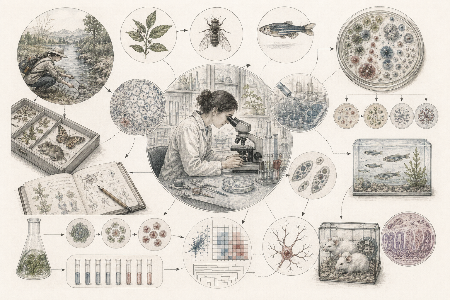
The article develops biological inquiry across natural history, laboratory experimentation, field ecology, molecular biology, microbiology, physiology, evolutionary reconstruction, conservation biology, marine biology, biotechnology, biomedical research, environmental monitoring, assay development, genomic analysis, imaging workflows, and computational reproducibility. It emphasizes that biological rigor comes not from reducing life to simplicity, but from designing methods that can handle variation, context, uncertainty, historical contingency, and multi-scale interaction.
The article also extends biological method into quantitative and computational practice through growth modeling, logistic dynamics, dose-response functions, assay validation, sensitivity and specificity, experimental design, replication, confidence intervals, sequence matching, imaging summaries, R workflows, Python workflows, SQL provenance structures, and a linked full-stack GitHub repository containing Python, R, Julia, Fortran, Rust, Go, C, C++, SQL, notebooks, data files, validation notes, and reproducibility documentation.
Biology and the problem of method
Biology studies living systems, but living systems are unusually difficult objects of inquiry. They are variable rather than uniform, historical rather than timeless, interactive rather than isolated, and organized across multiple levels of scale. A cell, a forest, a bacterial population, a coral reef, a microbial mat, and an animal nervous system do not present the same scientific problems, even though all belong to biology. For that reason, biological inquiry has never depended on one single method alone. It requires a plural methodology capable of moving between observation, experiment, comparison, historical reconstruction, statistical inference, modeling, and computation.
This methodological plurality reflects the nature of life itself. Biological systems grow, reproduce, mutate, cooperate, compete, develop, regulate, and change across time. They respond to environmental conditions, inherit structures shaped by earlier history, and often display nonlinear or context-dependent behavior. A science of life must therefore be able to identify patterns without assuming perfect uniformity, test causal claims without pretending complexity has disappeared, and reconstruct history where direct experiment is impossible.
Biology is rigorous not because it uses one privileged method, but because it brings multiple forms of evidence into disciplined relation. Observation reveals pattern. Experiment tests causal mechanisms. Comparison clarifies resemblance and difference. Classification stabilizes biological reference. Measurement gives variation numerical form. Statistics interprets uncertainty. Historical inference reconstructs deep time. Computation helps manage large datasets and complex systems. Together, these methods make biology a science of evidence under conditions of living complexity.
This also means that method is not secondary to biology. Method shapes what biology can know. A poorly designed field survey may miss species. A poorly controlled experiment may confuse causation. A poorly annotated dataset may become unusable. A poorly validated assay may generate misleading confidence. A model without transparent assumptions may clarify little. To understand biological inquiry is therefore to understand how knowledge of life is built, constrained, tested, and revised.
Observation as the foundation of biological knowledge
Observation is one of the oldest and most fundamental methods in biology. Before life could be modeled, manipulated, sequenced, or simulated, it had to be seen, described, distinguished, recorded, and compared. Natural history emerged through observation of plants, animals, habitats, bodily structures, life cycles, seasonal patterns, ecological relations, and geographic distributions. Even today, many important biological questions begin not in the laboratory but in attention to pattern: a trait that varies, a behavior that repeats, a population that declines, a disease that spreads, an organism that does not fit existing classification, or an ecological interaction that reveals hidden dependence.
Observation is not passive seeing. It is disciplined attention shaped by concepts, instruments, prior knowledge, and questions. A biologist observing a wetland, microscope slide, tissue section, microbial colony, field transect, electrophoresis gel, imaging plate, or sequencing readout is not merely looking. They are identifying relevant features, distinguishing signal from noise, recording regularities, and framing problems for further inquiry. Observation is therefore theory-informed, but not arbitrary. Good biological observation depends on training, explicit criteria, careful records, and openness to surprise.
In field biology, observation may involve transects, quadrats, camera traps, specimen collection, acoustic monitoring, remote sensing, mark-recapture protocols, phenology records, habitat surveys, and long-term ecological plots. In cell and molecular biology, observation may involve microscopy, staining, imaging, flow cytometry, sequencing, electrophoresis, protein assays, and live-cell tracking. In biotechnology, observation is often instrument-mediated through sensors, imaging systems, fluorescence signals, growth curves, optical density, bioassays, and automated pipelines.
The continuity across these settings is methodological. Biological observation identifies the variables, categories, anomalies, and patterns that later methods must explain. Without observation, experiment has no problem to test. Without observation, classification has no material to organize. Without observation, measurement has no biological meaning.
Experiment and the search for causation
If observation identifies patterns, experiment helps determine causes. Experimentation in biology attempts to manipulate conditions, isolate variables, compare treatment and control groups, and test whether specific factors influence particular outcomes. It allows biologists to move from correlation toward causal inference, asking not only what is associated with what, but what produces what under defined conditions. This has been especially important in physiology, genetics, microbiology, molecular biology, developmental biology, pharmacology, medicine, and biotechnology.
Yet biological experiment is often more difficult than experimental work in more tightly controlled physical systems. Organisms vary. Environments matter. Ethical constraints limit what can be manipulated. Many processes unfold over long timescales or involve interactions too complex to isolate completely. A laboratory experiment can provide precision, but may simplify away ecological context. A field experiment can preserve realism, but may involve more uncontrolled variation. Biological method must therefore balance control, realism, replication, and interpretation.
Experimental design is central to that balance. Randomization helps prevent systematic bias. Replication helps estimate variation. Controls help distinguish treatment effects from background processes. Blinding may reduce observer bias. Power analysis can help determine whether a study is likely to detect meaningful effects. Standardized protocols support reproducibility. Careful metadata make results interpretable after the experiment is complete.
In biotechnology, experiment often becomes platform-based. Researchers may perturb gene expression, compare treatment and control conditions, optimize fermentation parameters, screen cell lines, test antimicrobial susceptibility, validate biosensors, benchmark assay sensitivity and specificity, or compare sequencing pipelines. These are still biological experiments in the classical sense, but they are often coupled to instrumentation, statistics, automation, and reproducible workflows intended to support scalability and deployment.
Comparison, classification, and biological pattern
Biology has always depended on comparison. Organisms are compared to identify similarities, differences, homologies, analogies, and patterns of relation. Anatomical structures can be compared across species, behaviors across populations, genomes across lineages, microbial communities across habitats, and physiological responses across treatments. Comparison makes it possible to detect regularity in the midst of diversity and to ask whether resemblance reflects shared ancestry, convergent adaptation, common constraint, environmental plasticity, or functional necessity.
Classification is a formal extension of this comparative impulse. Taxonomy and systematics organize biological diversity into meaningful frameworks, making it possible to identify organisms, trace relatedness, and study life as an ordered field rather than an unstructured mass of particular cases. Classification has changed dramatically over time, especially with the rise of phylogenetic thinking, molecular data, and biodiversity informatics, but its scientific role remains crucial.
Comparison is also central to experimental interpretation. A treatment means little without a comparison group. A growth curve means little without a baseline. A pathogen sequence means little without reference data. A conservation trend means little without earlier records or comparable sites. Biology makes claims through difference, contrast, similarity, and relation.
Biotechnology depends on this comparative logic in practical ways. Sequence matching, microbial strain identification, biomarker discrimination, taxonomic assignment, cell-state classification, protein-domain comparison, and reference-database search all rely on comparison. A sequencing workflow that cannot distinguish taxa, strains, variants, or cell states is not merely inconvenient; it is methodologically weak. Comparative structure remains central even when it is mediated by databases and software rather than by visible morphology alone.
Measurement, quantification, and statistical inference
Modern biology increasingly depends on measurement. Traits are measured, populations counted, growth rates estimated, sequences aligned, biomarkers quantified, cells imaged, gene expression profiled, metabolic fluxes inferred, and ecological variables recorded across time and space. Measurement gives biology precision, allowing observed patterns to be described numerically rather than impressionistically. This matters because living systems vary, and variation must often be measured before it can be explained.
But measurement alone is not enough. Biological data are often noisy, incomplete, heterogeneous, and shaped by multiple influences at once. Statistical inference therefore plays a vital role in biological inquiry. It helps biologists assess uncertainty, test hypotheses, estimate relationships, interpret variability, compare models, and distinguish meaningful effects from random fluctuation. Probability and statistics are especially important because biological systems rarely behave as perfectly uniform mechanisms.
This quantitative turn has transformed biology. Experimental design, regression, survival analysis, population modeling, phylogenetic inference, biodiversity metrics, epidemiological estimation, dose-response modeling, high-throughput screening, genomic analysis, and environmental monitoring all depend on statistical reasoning. In biotechnology, the same logic governs assay calibration, dose-response estimation, quality control, classification thresholds, and validation of measurement pipelines.
Good measurement also requires attention to units, calibration, uncertainty, detection limits, sampling design, instrument drift, missing data, normalization, and data provenance. A number is not automatically evidence. It becomes evidence when its biological meaning, measurement process, uncertainty, and interpretive context are clear.
Field methods, laboratory methods, and multi-scale inquiry
Biological inquiry takes place in many settings because life itself exists across many settings. Field methods are essential for studying organisms in their environments, including behavior, ecological interaction, biodiversity, migration, habitat use, phenology, species distributions, disturbance response, and conservation status. Field biology captures the living world under real conditions, where context is not stripped away but treated as part of the phenomenon.
Laboratory methods, by contrast, offer greater control. Cells can be cultured, genes manipulated, molecules sequenced, tissues imaged, and physiological responses measured under defined conditions. Laboratory biology makes it possible to isolate mechanisms in ways that field inquiry often cannot. It has been especially decisive in microbiology, molecular biology, cell biology, genetics, physiology, biochemistry, and biomedicine.
The strongest biological research often moves between field and laboratory. Field observations may generate hypotheses that are tested experimentally. Laboratory findings may be evaluated under more realistic environmental conditions. Environmental samples may be sequenced and analyzed through bioinformatics. Clinical or ecological specimens may be transformed into controlled assays. Conservation questions may require both population surveys and genetic analysis.
Biotechnology often sits precisely at this junction. It may begin with field-derived samples, environmental isolates, agricultural materials, clinical specimens, or marine microbial communities, then move into laboratory pipelines for culturing, extraction, sequencing, screening, measurement, and computational interpretation. Robust workflows preserve the strengths of both domains: ecological or real-world relevance from field context, and mechanistic or analytical precision from laboratory control.
Historical inference and evolutionary reconstruction
Not all biological questions can be answered through direct experiment. Many concern events or processes that occurred in the past: the diversification of lineages, the emergence of traits, the timing of extinctions, the spread of populations, the origin of pathogens, or the deep history of life on Earth. Biology is therefore also a historical science. It often reconstructs what happened by drawing inferences from present traces, fossil evidence, comparative anatomy, molecular sequences, developmental structures, biogeographic distribution, and phylogenetic relationships.
This historical dimension is especially important in evolutionary biology, paleobiology, systematics, and comparative genomics, but it extends more broadly. The structure of a present organism often reflects prior evolutionary history. Disease susceptibility may depend on inherited biological legacies. Ecosystems bear marks of earlier disturbance, colonization, climate shifts, and human land use. A present biological pattern may therefore be unintelligible without a historical explanation.
Historical inference has its own standards. It does not simply speculate about the past. It compares evidence, tests alternative hypotheses, uses phylogenetic models, estimates divergence, examines fossil sequences, and evaluates whether present patterns are more consistent with one historical scenario than another. The past cannot always be experimentally repeated, but it can be scientifically inferred.
Biotechnology also uses historical inference, especially through comparative genomics, phylogenetics, and sequence-based lineage tracing. Whether one is reconstructing the spread of a pathogen, inferring the ancestry of a microbial strain, or identifying a sequence variant relative to a reference panel, the logic is the same: present data are interpreted as traces of prior biological history.
Ecological, marine, and environmental methods
Ecology, marine biology, and environmental biology require methods that can handle complexity at landscape, watershed, coastal, oceanic, and ecosystem scales. These fields study organisms in context: interacting with other organisms, physical conditions, chemical gradients, climate variation, nutrient availability, habitat structure, disturbance, and human pressure. Their methods therefore often combine observation, measurement, experimental manipulation, remote sensing, statistical modeling, and long-term monitoring.
Ecological methods may include quadrat sampling, transects, mark-recapture, occupancy modeling, stable-isotope analysis, biodiversity surveys, environmental DNA sampling, acoustic monitoring, sensor networks, experimental plots, and satellite imagery. Marine methods may include plankton tows, benthic surveys, coral health assessment, autonomous sensors, oceanographic sampling, underwater imaging, metabarcoding, and carbonate chemistry measurement. Environmental monitoring may track water quality, soil health, air pollutants, microbial contamination, nutrient flux, ecosystem recovery, or species distributions.
These methods matter because ecological and marine systems are often too large, dynamic, and heterogeneous for simple laboratory reduction. A coral reef, wetland, forest, estuary, microbial mat, or coastal fishery cannot be fully understood through one measurement. It requires multiple indicators across time and space. Methodological rigor therefore depends on sampling design, instrument calibration, spatial coverage, temporal replication, metadata, and statistical treatment of uncertainty.
Environmental methods also carry ethical and governance implications. Biodiversity monitoring, conservation planning, pollution assessment, and restoration ecology are not merely academic exercises. They guide decisions about land, water, species protection, community health, and intergenerational responsibility. Strong biological method is therefore part of responsible environmental knowledge.
Biomedical and biotechnology methods
Biomedicine and biotechnology make biological method operational. Observation becomes microscopy, imaging, sensor capture, sequencing, cytometry, assay readout, and clinical measurement. Experiment becomes controlled perturbation, screening, treatment comparison, gene editing, pathway manipulation, microbial growth testing, and platform optimization. Classification becomes database-backed identification. Measurement becomes assay validation. Statistical inference becomes essential for deciding whether a signal is real, reproducible, clinically relevant, or actionable.
Biomedical methods must handle variability at many levels: genetic background, cell state, tissue context, disease stage, immune response, microbiome composition, treatment exposure, and environmental condition. Biotechnology adds additional concerns: production reproducibility, contamination control, batch effects, sensitivity, specificity, limit of detection, dynamic range, signal-to-noise ratio, throughput, and quality control.
This makes biotechnology a strong example of method-intensive biology. Fermentation, environmental sequencing, microbial remediation, biomaterials, agricultural biology, biosensor development, wastewater monitoring, conservation genomics, and high-throughput screening all depend on robust biological method. The applied setting may differ from classical natural history or laboratory biology, but the methodological core remains the same: disciplined inference from biological evidence under conditions of uncertainty and variation.
In that sense, biotechnology does not replace basic biology. It operationalizes it. The more sophisticated the workflow becomes, the more it depends on strong foundations in observation, experimental design, comparison, statistical reasoning, measurement validation, and computational transparency.
Reproducibility, provenance, and open biological workflows
Modern biological method increasingly requires reproducibility and provenance. A result is stronger when another researcher can understand how the data were collected, how the samples were handled, how measurements were processed, how code was run, how parameters were chosen, and how conclusions were drawn. Reproducibility does not mean every biological result will be identical in every context. Living systems vary. But it does mean that methods should be transparent enough to evaluate, repeat, audit, and improve.
Provenance is especially important in data-rich biology. A sequence read, image file, specimen record, cell-count table, sensor output, or ecological observation should be linked to metadata: who collected it, when, where, with what instrument or protocol, under what conditions, and with what processing steps. Without provenance, data lose interpretability. A spreadsheet of numbers without sampling context may be unusable. A sequence without metadata may be difficult to validate. An image without acquisition details may be hard to compare.
Open workflows support this methodological discipline. Version-controlled code, documented datasets, structured metadata, notebooks, containerized environments, validation checks, and clear licensing can make biological research more transparent. Open methods do not eliminate error, but they make errors easier to find. They also allow others to extend, critique, and reuse biological work.
This is why computational biology is not merely a technical add-on. It is increasingly part of the epistemic infrastructure of biology: the system through which evidence becomes traceable, reviewable, reproducible, and open to correction.
Mathematical lens
As biology has become more quantitative, mathematics and computation have become increasingly important parts of biological method. Population growth can be modeled mathematically. Inheritance can be described probabilistically. Disease transmission can be simulated dynamically. Assays can be validated statistically. Sequence matching can be automated. Imaging workflows can extract features from thousands of cells. In each case, mathematical structure helps clarify processes that are otherwise too complex, large-scale, or nonlinear to grasp intuitively.
For a microbial or cellular population under unconstrained early growth, one common model is:
Interpretation: Exponential growth describes population increase when the per-capita growth rate remains constant.
where \(N_0\) is the initial abundance, \(r\) is the per-capita growth rate, and \(t\) is time. This model converts raw abundance observations into interpretable parameters such as growth rate and doubling time:
Interpretation: Doubling time converts a growth rate into the time required for abundance to double.
If growth becomes resource-limited, a logistic model is often more appropriate:
Interpretation: Logistic growth represents population increase under carrying-capacity limitation.
where \(K\) is the carrying capacity. This model is directly useful in microbial biotechnology, fermentation, cell culture, ecological monitoring, algal growth, and population biology.
Many biotech workflows involve treatment effects, inhibition curves, or assay-response modeling. A common sigmoidal form is the Hill equation:
Interpretation: The Hill equation models how biological effect changes with concentration.
where \(E(c)\) is effect at concentration \(c\), \(EC_{50}\) is the half-maximal effective concentration, and \(n\) is the Hill coefficient. This form is useful in antimicrobial testing, enzyme inhibition, receptor biology, toxicology, pharmacology, and screening assays.
Biological methods often require validation against known conditions. Sensitivity and specificity are basic measures:
Interpretation: Sensitivity measures the share of true positive cases correctly detected by an assay.
Interpretation: Specificity measures the share of true negative cases correctly identified by an assay.
where \(TP\) is true positives, \(FN\) is false negatives, \(TN\) is true negatives, and \(FP\) is false positives. These measures matter in diagnostics, biosurveillance, environmental testing, microbial detection, and assay validation.
When repeated measurements are available, a simple confidence interval for a sample mean is:
Interpretation: A confidence interval expresses uncertainty around an estimated mean using sample variation and sample size.
where \(\bar{x}\) is the sample mean, \(s\) is sample standard deviation, \(n\) is sample size, and \(t\) is the relevant critical value. This does not eliminate uncertainty, but it expresses uncertainty quantitatively.
Variables, units, and methodological interpretation
Biological method depends on variables that connect observation, experiment, measurement, uncertainty, and interpretation. The table below summarizes several central quantities used in introductory quantitative biological inquiry.
| Symbol or Term | Meaning | Typical Unit or Scale | Methodological Interpretation |
|---|---|---|---|
| \(N\) | Abundance or population size | cells, organisms, colonies, reads, biomass proxy, or count | Measured biological quantity used to track growth, decline, or sample composition |
| \(N_0\) | Initial abundance | same as \(N\) | Starting condition for growth models or experimental comparisons |
| \(t\) | Time | seconds, hours, days, years, or generations | Temporal dimension over which biological change is observed |
| \(r\) | Per-capita growth rate | per unit time | Estimated rate of biological increase under specified conditions |
| \(K\) | Carrying capacity | same as \(N\) | Approximate upper abundance supported by limiting conditions |
| \(t_d\) | Doubling time | time | Time required for abundance to double under an estimated growth rate |
| \(c\) | Concentration | molarity, mass per volume, dose, or assay-specific unit | Input level used in dose-response or treatment-effect experiments |
| \(EC_{50}\) | Half-maximal effective concentration | same as \(c\) | Concentration associated with half-maximal biological response |
| \(TP, FN, TN, FP\) | Validation outcomes | counts | True positives, false negatives, true negatives, and false positives in assay evaluation |
| \(\bar{x}\) | Sample mean | same as measured variable | Central estimate from repeated measurements |
| \(s\) | Sample standard deviation | same as measured variable | Observed variation among repeated measurements |
| \(n\) | Sample size | count | Number of observations contributing to an estimate |
The table illustrates why method matters in biology. Biological variables are not only mathematical symbols. They are tied to sampling decisions, instrument readings, experimental design, metadata, uncertainty, and interpretation.
Worked example: growth rate and doubling time
Suppose a microbial culture begins with \(N_0=1.0\times10^5\) cells and reaches \(1.0\times10^6\) cells after 10 hours. Under the exponential model:
Interpretation: Exponential growth relates abundance to initial abundance, growth rate, and elapsed time.
Substituting the observed values gives:
Interpretation: The observed change in cell abundance can be used to estimate the growth rate.
Dividing both sides by \(1.0\times10^5\):
Interpretation: The culture increased tenfold over the observation period.
Taking the natural logarithm of both sides:
Interpretation: The estimated growth rate is approximately 0.2303 per hour.
The doubling time is:
Interpretation: At this estimated rate, the population doubles about every 3.01 hours.
This simple calculation converts observed growth into interpretable biological parameters. It also shows why method and mathematics belong together: the biological observation becomes useful only when its assumptions, time interval, units, and inferential logic are clear.
Computational modeling
Computational modeling helps make biological method explicit. Growth curves can be fitted to observational or experimental data. Logistic models can compare treatment conditions, resource limitation, or carrying capacity. Assay validation metrics can be computed from diagnostic outcomes. Sequence matching can classify biological samples against reference data. Imaging features can be summarized from cell-level measurements. Metadata and provenance structures can preserve how evidence was produced.
The selected examples below focus on compact but reusable workflows: growth-curve fitting, assay validation, logistic simulation, sequence matching, and imaging feature summaries. The GitHub repository extends the same logic into richer computational scaffolding: dose-response models, experimental design metadata, validation tables, SQL provenance structures, notebooks, documentation, sample data, and multi-language implementations.
The purpose is not to substitute computation for biological judgment. It is to make the evidence chain more inspectable. In biological inquiry, a model is strongest when its assumptions are visible, its data are documented, and its outputs can be checked.
R workflow: growth curves and assay validation
R is especially useful for biological method because it supports statistical modeling, tabular reporting, reproducible analysis, and transparent summaries. The following workflow estimates an exponential growth rate from biological count data and calculates basic assay validation metrics.
# Growth Curves and Assay Validation
#
# This workflow demonstrates two common biological-method tasks:
#
#   1. Fit an exponential growth model from count data.
#   2. Summarize sensitivity, specificity, and predictive values
#      for a diagnostic, biosurveillance, or screening assay.
#
# Replace the synthetic values with microbial, cellular, algal,
# environmental monitoring, clinical, or biotechnology observations.

library(tibble)
library(dplyr)

# ------------------------------------------------------------
# 1. Fit an exponential growth model from biological count data
# ------------------------------------------------------------

growth_data <- tibble(
  time_h = c(0, 2, 4, 6, 8, 10),
  cells = c(1.0e5, 1.6e5, 2.7e5, 4.3e5, 6.8e5, 1.0e6)
)

growth_model <- lm(log(cells) ~ time_h, data = growth_data)

growth_summary <- tibble(
  growth_rate_per_h = coef(growth_model)[["time_h"]],
  estimated_initial_abundance = exp(coef(growth_model)[["(Intercept)"]]),
  doubling_time_h = log(2) / growth_rate_per_h,
  r_squared_log_space = summary(growth_model)$r.squared
)

growth_predictions <- growth_data %>%
  mutate(
    predicted_cells = exp(predict(growth_model)),
    residual_log_scale = resid(growth_model)
  )

# ------------------------------------------------------------
# 2. Simple diagnostic or biosurveillance assay validation table
# ------------------------------------------------------------

validation_counts <- tibble(
  true_positive = 84,
  false_negative = 16,
  true_negative = 91,
  false_positive = 9
)

validation_summary <- validation_counts %>%
  mutate(
    sensitivity = true_positive / (true_positive + false_negative),
    specificity = true_negative / (true_negative + false_positive),
    positive_predictive_value = true_positive / (true_positive + false_positive),
    negative_predictive_value = true_negative / (true_negative + false_negative)
  )

print(round(growth_summary, 5))
print(round(growth_predictions, 3))
print(round(validation_summary, 4))
This workflow turns assay or culture measurements into interpretable growth parameters and validation metrics. A scientist could extend it to treatment comparisons, confidence intervals, nonlinear logistic fits, batch-effect correction, calibration analysis, or quality-control dashboards.
Python workflow: logistic growth, sequence matching, and imaging summaries
Python is especially useful for simulation, data pipelines, bioinformatics, imaging workflows, and reproducible biological analysis. The following workflow compares logistic growth scenarios, performs a simple sequence-matching task, and summarizes image-derived cellular features.
"""
Biological Methods Workflow

This workflow demonstrates three common computational tasks
in biological inquiry:

1. Simulate logistic growth under different biological conditions.
2. Match a query sequence against aligned reference sequences.
3. Summarize image-derived cellular features by condition.

The examples are intentionally compact, but the same structure can be
extended into microbial biotechnology, environmental monitoring,
cell-imaging workflows, pathogen surveillance, assay validation,
or reproducible biological data pipelines.
"""

from __future__ import annotations

import numpy as np
import pandas as pd

def logistic_growth(
    time: np.ndarray,
    initial_abundance: float,
    growth_rate: float,
    carrying_capacity: float,
) -> np.ndarray:
    """
    Calculate a logistic growth trajectory.
    """
    if initial_abundance <= 0:
        raise ValueError("Initial abundance must be positive.")
    if carrying_capacity <= 0:
        raise ValueError("Carrying capacity must be positive.")
    if initial_abundance > carrying_capacity:
        raise ValueError("Initial abundance should not exceed carrying capacity.")

    return carrying_capacity / (
        1.0
        + ((carrying_capacity - initial_abundance) / initial_abundance)
        * np.exp(-growth_rate * time)
    )

def hamming_distance(seq1: str, seq2: str) -> int:
    """
    Calculate Hamming distance for two aligned equal-length sequences.
    """
    if len(seq1) != len(seq2):
        raise ValueError("Sequences must be aligned and equal length.")

    return sum(a != b for a, b in zip(seq1, seq2))

def summarize_logistic_growth() -> pd.DataFrame:
    """
    Simulate logistic growth under multiple scenarios.
    """
    time_h = np.linspace(0, 24, 300)

    scenarios = {
        "baseline": {"N0": 1.0e5, "r": 0.45, "K": 2.0e6},
        "nutrient_limited": {"N0": 1.0e5, "r": 0.25, "K": 9.0e5},
        "treatment": {"N0": 1.0e5, "r": 0.12, "K": 5.0e5},
    }

    rows = []

    for scenario, params in scenarios.items():
        abundance = logistic_growth(
            time=time_h,
            initial_abundance=params["N0"],
            growth_rate=params["r"],
            carrying_capacity=params["K"],
        )

        rows.append(
            pd.DataFrame(
                {
                    "scenario": scenario,
                    "time_h": time_h,
                    "abundance": abundance,
                    "growth_rate": params["r"],
                    "carrying_capacity": params["K"],
                }
            )
        )

    return pd.concat(rows, ignore_index=True)

def match_query_sequence() -> pd.DataFrame:
    """
    Match a query sequence against aligned references.
    """
    reference = {
        "strain_A": "ATGCTAGCTAAC",
        "strain_B": "ATGCTAGCTATC",
        "strain_C": "ATGCCAGCTATC",
    }

    query = "ATGCTAGCTATC"

    rows = []

    for name, sequence in reference.items():
        distance = hamming_distance(query, sequence)
        similarity = 1.0 - distance / len(query)

        rows.append(
            {
                "candidate": name,
                "hamming_distance": distance,
                "similarity": similarity,
            }
        )

    return pd.DataFrame(rows).sort_values(
        ["hamming_distance", "candidate"],
        ascending=[True, True],
    )

def summarize_cell_images() -> pd.DataFrame:
    """
    Summarize image-derived cellular features by condition.
    """
    cells = pd.DataFrame(
        {
            "cell_id": ["cell_001", "cell_002", "cell_003", "cell_004", "cell_005"],
            "condition": ["control", "control", "treated", "treated", "treated"],
            "area_um2": [820, 790, 640, 610, 660],
            "mean_intensity": [1450, 1390, 1180, 1110, 1205],
            "roundness": [0.74, 0.76, 0.68, 0.66, 0.69],
        }
    )

    return (
        cells.groupby("condition")
        .agg(
            n_cells=("cell_id", "count"),
            mean_area_um2=("area_um2", "mean"),
            mean_intensity=("mean_intensity", "mean"),
            mean_roundness=("roundness", "mean"),
        )
        .reset_index()
    )

def main() -> None:
    """
    Run compact examples for growth modeling, sequence matching,
    and imaging-feature summaries.
    """
    growth_df = summarize_logistic_growth()
    matches = match_query_sequence()
    image_summary = summarize_cell_images()

    print("Logistic growth sample:")
    print(growth_df.head(12).round(3).to_string(index=False))

    print("\nBest sequence match:")
    print(matches.to_string(index=False))
    print("Best match:", matches.iloc[0]["candidate"])

    print("\nImaging feature summary:")
    print(image_summary.round(3).to_string(index=False))

if __name__ == "__main__":
    main()
This Python workflow reflects three increasingly common forms of modern biological method. Growth models help compare biological conditions. Sequence matching supports classification, surveillance, and molecular identification. Imaging summaries convert visual observations into structured, analyzable evidence.
GitHub repository
The article body includes compact R and Python examples so the scientific argument remains readable. The full repository expands those examples into a more rigorous computational biological-methods workflow, including growth-curve modeling, logistic simulation, dose-response scaffolding, assay validation, sensitivity and specificity calculation, sequence matching, imaging feature summaries, experimental design metadata, SQL provenance structures, validation notes, reproducible data files, and full-stack scientific-computing examples across Python, R, Julia, Fortran, Rust, Go, C, C++, SQL, and notebooks.
Limits, complexity, and the ethics of biological inquiry
Biological inquiry faces limits because living systems are complex and because not all questions can be pursued without constraint. Organisms are not inert objects. They have welfare, ecological roles, evolutionary histories, and relationships to human communities. Experiments involving animals, ecosystems, pathogens, Indigenous lands, endangered species, or human biological materials raise ethical questions that cannot be treated as external to method. The means by which biology acquires knowledge are part of the moral structure of the science.
Complexity imposes additional limits. A result obtained in one model organism may not generalize fully to another. A laboratory effect may not scale to ecosystems. A statistically significant result may still have limited explanatory power if the underlying system is highly context-dependent. A machine-learning classifier may perform well on one dataset and poorly on another. A sequencing pipeline may produce confident but incorrect assignments if the reference database is incomplete.
In biotechnology, the same caution applies to pipeline performance, sequence assignment, screening assays, predictive modeling, biosafety, and environmental deployment. A biological intervention can have consequences beyond the immediate assay or system. Methodological rigor therefore includes ethical awareness, risk assessment, transparency, and humility about uncertainty.
This is one reason reproducibility, provenance, and critical evaluation matter so much. Biological methods must not only produce results; they must make those results contestable, reviewable, and open to refinement. A method that cannot be checked is weaker than one that can be challenged.
Why biological methods matter
The methods of biological inquiry matter because biological knowledge shapes medicine, public health, agriculture, conservation, environmental policy, biotechnology, and planetary stewardship. Decisions about disease control, genetic testing, ecological restoration, food systems, biosurveillance, biodiversity protection, and climate adaptation depend on whether biological evidence has been generated and interpreted well. Method is therefore not a technical detail beneath the surface of biology. It is part of what makes biological claims trustworthy.
Methods also matter because the living world is changing rapidly. Climate disruption, habitat fragmentation, extinction, emerging disease, pollution, land-use change, and the expansion of data-intensive biology all require methods capable of detecting change, interpreting complexity, and producing knowledge that can guide action under uncertainty. Biotechnology magnifies this need because it often moves biological insight toward intervention, production, monitoring, or governance.
To understand how biology knows is therefore part of understanding what biology is. The science of life is also a science of evidence, method, uncertainty, and disciplined inference. Its credibility depends not only on what it studies, but on how it studies it.
Conclusion
Observation, experiment, and the methods of biological inquiry show that biology is not defined by one single procedure, but by a family of rigorous approaches adapted to the complexity of life. Observation identifies pattern. Experiment tests causation. Comparison and classification organize diversity. Measurement and statistics interpret variation. Historical reconstruction explains deep time. Mathematics and computation extend biological reasoning into systems, models, and large datasets.
This plurality is not a weakness. It is a consequence of biology’s subject matter. Living systems are organized, variable, interactive, and historical. They require a science capable of moving between field and laboratory, mechanism and history, description and model, organism and system. Biotechnology inherits and intensifies these demands by translating biological knowledge into screening workflows, sequencing pipelines, assay systems, environmental monitoring, and reproducible computational analysis.
To study biological inquiry is therefore to see how knowledge of life is built: patiently, comparatively, experimentally, quantitatively, historically, ethically, and under conditions of complexity. Biology advances not because life is simple, but because scientific method makes complexity progressively more intelligible.
Related articles
- Biology
- What Is Biology?
- Biology and the Scientific Understanding of Living Order
- The Rise of Modern Biological Thought
- Classification, Taxonomy, and the Ordering of Life
- Cell Theory and the Basic Unit of Life
- Life, Death, and the Problem of Biological Definition
- Ecology and the Interdependence of Life
- Conservation Biology and the Protection of Life
- Systems Biology and the Logic of Biological Integration
Further reading
- Altman, D.G. and Bland, J.M. (1994) ‘Diagnostic tests 1: Sensitivity and specificity’, BMJ, 308, p. 1552. Available at: https://www.bmj.com/content/308/6943/1552
- Fisher, R.A. (1935) The Design of Experiments. Edinburgh: Oliver and Boyd. Available at: https://archive.org/details/designofexperime00fish
- Gotelli, N.J. and Ellison, A.M. (2013) A Primer of Ecological Statistics. 2nd edn. Sunderland, MA: Sinauer Associates.
- Mayr, E. (1982) The Growth of Biological Thought: Diversity, Evolution, and Inheritance. Cambridge, MA: Harvard University Press.
- National Academies of Sciences, Engineering, and Medicine (2019) Reproducibility and Replicability in Science. Washington, DC: National Academies Press. Available at: https://nap.nationalacademies.org/catalog/25303/reproducibility-and-replicability-in-science
- National Research Council (2003) BIO2010: Transforming Undergraduate Education for Future Research Biologists. Washington, DC: National Academies Press. Available at: https://nap.nationalacademies.org/catalog/10497/bio2010-transforming-undergraduate-education-for-future-research-biologists
- OpenStax (2018) ‘The process of science’, in Biology 2e. Available at: https://openstax.org/books/biology-2e/pages/1-2-the-process-of-science
- Sober, E. (2008) Evidence and Evolution: The Logic Behind the Science. Cambridge: Cambridge University Press.
- Wickham, H., Çetinkaya-Rundel, M. and Grolemund, G. (2023) R for Data Science. 2nd edn. Available at: https://r4ds.hadley.nz/
References
- Altman, D.G. and Bland, J.M. (1994) ‘Diagnostic tests 1: Sensitivity and specificity’, BMJ, 308, p. 1552. Available at: https://www.bmj.com/content/308/6943/1552
- Fisher, R.A. (1935) The Design of Experiments. Edinburgh: Oliver and Boyd. Available at: https://archive.org/details/designofexperime00fish
- Gotelli, N.J. and Ellison, A.M. (2013) A Primer of Ecological Statistics. 2nd edn. Sunderland, MA: Sinauer Associates.
- Mayr, E. (1982) The Growth of Biological Thought: Diversity, Evolution, and Inheritance. Cambridge, MA: Harvard University Press.
- National Academies of Sciences, Engineering, and Medicine (2019) Reproducibility and Replicability in Science. Washington, DC: National Academies Press. Available at: https://nap.nationalacademies.org/catalog/25303/reproducibility-and-replicability-in-science
- National Research Council (2003) BIO2010: Transforming Undergraduate Education for Future Research Biologists. Washington, DC: National Academies Press. Available at: https://nap.nationalacademies.org/catalog/10497/bio2010-transforming-undergraduate-education-for-future-research-biologists
- OpenStax (2018) ‘The process of science’, in Biology 2e. Available at: https://openstax.org/books/biology-2e/pages/1-2-the-process-of-science
- OpenStax (2018) ‘The study of life’, in Biology 2e. Available at: https://openstax.org/books/biology-2e/pages/1-1-themes-and-concepts-of-biology
- Sober, E. (2008) Evidence and Evolution: The Logic Behind the Science. Cambridge: Cambridge University Press.
- Wickham, H., Çetinkaya-Rundel, M. and Grolemund, G. (2023) R for Data Science. 2nd edn. Available at: https://r4ds.hadley.nz/