
Last Updated May 12, 2026
Edge analytics and local data processing examine how embedded and edge systems transform raw local data into timely, selective, and operationally meaningful outputs before those data are sent elsewhere. In embedded systems, edge analytics is not simply cloud analytics moved outward. It is the architectural discipline of placing filtering, aggregation, stream processing, feature extraction, inference, anomaly detection, buffering, replay handling, and selective uplink near the point of sensing or action so that systems respond faster, transmit less, preserve continuity, and remain interpretable under imperfect connectivity.
Many embedded systems generate more data than can or should be transmitted upstream in raw form. Cameras, vibration sensors, industrial telemetry, environmental streams, wearable signals, acoustic monitors, robotics logs, and operational traces can produce high-volume local information continuously. Yet only a fraction of that information is immediately relevant to decision-making. Edge analytics exists because transmitting everything is often too slow, too expensive, too bandwidth-intensive, too privacy-sensitive, too energy-consuming, or too fragile under real-world connectivity constraints.
This means local data processing is not merely a transport optimization. It is a decision about where meaning is created. A system that performs threshold detection, rolling-window aggregation, feature extraction, event qualification, anomaly scoring, alert generation, local inference, raw-window retention, or selective export at the edge is deciding that some interpretations should exist before cloud-scale storage or analysis ever begins.
The deeper architectural question is therefore not whether analytics can happen at the edge, but which analytics should happen there, under what constraints, with what lineage preserved, and with what relationship to upstream systems. Edge analytics becomes strongest when local processing improves responsiveness and resilience without making system logic opaque, fragmenting interpretability, or hiding the conditions under which local meaning was produced.
Main Library
Publications
Article Map
Embedded & Edge Systems
Related Topic
Data Systems & Analytics
Related Topic
Artificial Intelligence Systems
Related Topic
Intelligent Infrastructure
For engineers, edge analytics should be treated as a managed analytical layer, not as incidental preprocessing. It determines what data are retained, what signals are reduced, what local events are declared meaningful, what gets forwarded upstream, what remains only at the edge, and how downstream systems should interpret delayed, summarized, or inferred outputs. A local analytics layer that reduces bandwidth but destroys timing, lineage, freshness, quality context, or replay evidence can make the system faster while making it less trustworthy.
Engineering Problem
The engineering problem is how to transform high-rate, heterogeneous, locally generated data into useful operational signals without exceeding device, gateway, bandwidth, storage, privacy, energy, or latency constraints. Edge analytics must decide what should be processed locally, what should be preserved for later review, what should be summarized, what should be transmitted immediately, what can wait, and what can be safely discarded.
This is not merely a data-reduction problem. Edge analytics changes the meaning of the data that downstream systems receive. A cloud platform may never see the original signal, only a feature vector, rolling statistic, alarm, anomaly score, classification result, or backfilled local summary. That means local processing becomes part of the system’s epistemic chain: what the wider system can know depends on what the edge layer sensed, transformed, retained, and disclosed.
Weak edge analytics pipelines often fail by hiding this transformation. They compute useful local summaries but do not preserve acquisition time. They detect anomalies but do not record the threshold, window, feature version, rule version, or model version that produced the result. They reduce bandwidth but make forensic reconstruction impossible. They buffer data but allow delayed outputs to appear current. They perform inference but mix raw, derived, rule-based, and model-based values into one undifferentiated stream.
The practical question is therefore: can the system create timely local meaning while preserving enough lineage, freshness, quality, replay, and decision context for upstream systems, operators, and engineers to interpret the results honestly?
Reference Architecture
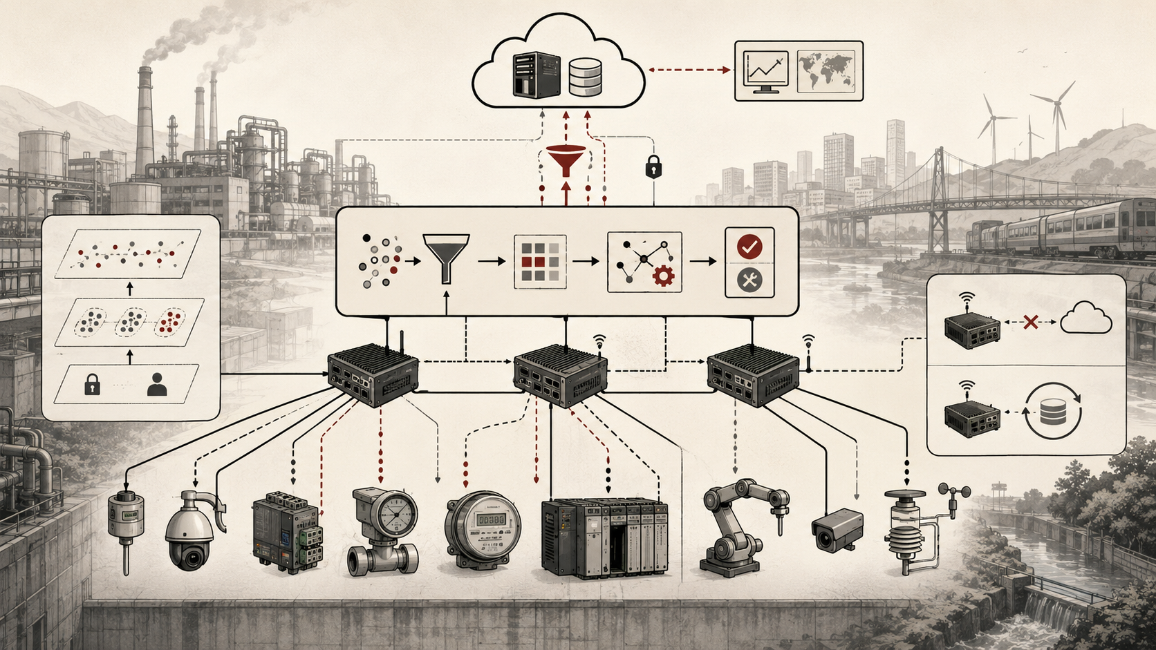
A practical edge analytics architecture can be understood as a local analytical pipeline connected to wider data systems. The implementation may involve microcontrollers, gateways, stream processors, local databases, message brokers, edge runtimes, cloud IoT platforms, industrial historians, TinyML runtimes, PYNQ overlays, SQL engines, or custom services. The underlying responsibilities remain broadly consistent.
| Layer | Engineering Role | Edge Analytics Concern | Evidence Artifact |
|---|---|---|---|
| Acquisition layer | Collects raw signals from sensors, logs, controllers, cameras, microphones, or devices | Sampling, timestamping, calibration, sensor health, acquisition integrity | Sensor manifest, acquisition log, calibration record |
| Preprocessing layer | Cleans, filters, normalizes, resamples, denoises, or validates incoming signals | Numerical stability, unit consistency, missing data, outliers | Preprocessing manifest, validation log, unit map |
| Windowing layer | Groups stream data into tumbling, sliding, session, or event-driven windows | Reaction time, noise sensitivity, state retention, late data | Window policy, event-time record, watermark log |
| Feature and summary layer | Computes compact representations such as averages, counts, peaks, rates, spectra, or scores | Compression, interpretability, feature drift, signal loss | Feature schema, summary contract, reduction report |
| Event logic layer | Applies thresholds, rules, state machines, joins, and event qualification | False alarms, event semantics, temporal conditions, rule versions | Event contract, rule manifest, decision log |
| Local inference layer | Runs models or classifiers locally when needed | Model version, confidence, latency, runtime constraints, fallback logic | Model card, inference event, confidence record |
| Buffering and persistence layer | Retains raw windows, features, events, or summaries during outages or review windows | Retention, replay, freshness, priority, storage limits | Buffer policy, replay record, retention ledger |
| Selective uplink layer | Chooses which records move upstream immediately, later, or never | Bandwidth, privacy, cost, urgency, explainability | Forwarding policy, uplink log, drop reason |
| Observability layer | Tracks local pipeline health, freshness, quality, latency, backlog, and drift | Debugging, audit, field monitoring, incident reconstruction | Analytics health report, telemetry schema, SLO report |
| Cloud and fleet layer | Performs long-horizon storage, cross-site analysis, model training, and governance | Version control, fleet comparison, retraining, policy coordination | Fleet report, model registry, governance record |
This architecture makes local analytics visible as infrastructure. It separates acquisition from processing, processing from interpretation, interpretation from action, and local action from upstream governance. Without those distinctions, edge analytics can become a hidden transformation layer that accelerates decisions while weakening accountability.
Implementation Pattern
A rigorous edge analytics implementation begins by defining the signal, the operational need, the local constraints, the analytical transformation, the retention policy, the uplink policy, and the downstream interpretation contract. Engineers should specify not only what gets calculated locally, but why it belongs at the edge, how it is validated, what evidence is preserved, and what upstream systems are allowed to infer from it.
| Artifact | Purpose | Typical Format |
|---|---|---|
| Signal manifest | Defines source signals, units, sampling rate, calibration state, and expected quality | YAML, JSON, sensor inventory |
| Preprocessing contract | Defines filtering, normalization, missing-data handling, unit conversion, and validation rules | YAML, JSON Schema, SQL checks |
| Window policy | Defines window length, overlap, event-time semantics, watermarks, and late-data handling | YAML, stream config |
| Feature schema | Defines computed features, summaries, rates, counts, and signal reductions | JSON Schema, SQL table, CSV dictionary |
| Event logic manifest | Defines thresholds, temporal conditions, state transitions, event qualification, and rule versions | YAML, policy-as-code, stream SQL |
| Local inference manifest | Defines model version, runtime, input features, confidence threshold, and fallback behavior | Model card, YAML, runtime manifest |
| Buffer policy | Defines what raw windows, features, events, and summaries are retained and for how long | YAML, retention ledger |
| Selective uplink policy | Defines immediate, deferred, sampled, summarized, and suppressed transmission behavior | YAML, stream routing policy |
| Replay policy | Defines late data, ordering, duplicate handling, correction records, and backfill interpretation | YAML, stream contract, replay manifest |
| Analytics SLO | Defines freshness, latency, backlog, data-loss, feature completeness, and event-quality targets | YAML, monitoring config |
| Analytics event schema | Defines what the local analytics layer reports upstream | SQL, JSON Schema, telemetry schema |
The implementation goal is to make local meaning inspectable. Engineers should be able to reconstruct what was sensed, which local transformation was applied, what window produced the result, whether the result was fresh, what data were retained, what was forwarded, what was suppressed, and what local decision logic interpreted the output.
Research-Grade Framing: Edge Analytics as Local Meaning Infrastructure
Edge analytics should be framed as local meaning infrastructure. It is the layer where raw local data become operationally interpretable before they enter wider information systems. This matters because the first analytical transformation often determines what the rest of the architecture can know. A raw vibration waveform may become a rolling RMS score, an anomaly flag, a spectral feature, a retained incident window, or a discarded non-event. A camera stream may become a count, zone occupancy summary, event trigger, or local inference result. Each choice narrows and shapes the data lifecycle.
This framing prevents a common mistake: treating edge analytics as a neutral optimization. Local processing can reduce bandwidth, latency, storage, and exposure, but it also changes evidence. Once a signal is summarized, filtered, classified, or retained selectively, downstream systems inherit that transformation. If the transformation is not versioned, timestamped, validated, and observable, then local analytics may create faster outputs while making the system less intelligible.
| Evidence Dimension | Question | Required Edge Analytics Evidence |
|---|---|---|
| Input lineage | What raw signal or local stream produced the result? | Sensor ID, signal ID, acquisition time, calibration state |
| Transformation | Was the output raw, filtered, aggregated, inferred, or event-qualified? | Processing stage, feature schema, rule/model version |
| Window semantics | What time window or event condition produced the output? | Window ID, start/end time, watermark, late-data policy |
| Freshness | Is the output live, delayed, backfilled, or historical? | Acquisition time, processing time, uplink time, ingestion time |
| Quality | Were inputs missing, noisy, stale, invalid, or low confidence? | Quality flags, completeness score, sensor-health state |
| Retention | What raw or derived evidence remains available? | Retention policy, buffer status, raw-window pointer |
| Forwarding | Why was the output sent, retained, summarized, or dropped? | Selective uplink rule, priority, bandwidth state, drop reason |
A mature edge analytics system therefore does not only ask, “What did the edge compute?” It asks, “What did this local computation make knowable, what did it make invisible, and what evidence remains for later interpretation?”
Formal Model: Local Signals, Windows, Features, Events, and Uplink
A useful formal model separates local signals, preprocessing, windows, features, event logic, inference, buffering, and upstream transmission. Let \(x_t\) represent the raw local signal at time \(t\), \(P(\cdot)\) the preprocessing function, \(W_k\) a local window, \(\phi(\cdot)\) the feature function, \(E(\cdot)\) the event logic, and \(u_t\) the upstream output.
\tilde{x}_t = P(x_t, q_t, c_t)
\]
Interpretation: Preprocessed signal \(\tilde{x}_t\) depends on raw input \(x_t\), quality state \(q_t\), and calibration or configuration state \(c_t\). Local processing should preserve enough metadata to explain this transformation.
W_k = \{ \tilde{x}_t : t_k \leq t < t_k + \Delta \}
\]
Interpretation: Window \(W_k\) groups local stream values over duration \(\Delta\). Window design controls responsiveness, smoothing, event timing, and local memory requirements.
z_k = \phi(W_k)
\]
Interpretation: Feature vector \(z_k\) is computed from a local window. Edge analytics often reduces raw streams into compact, locally meaningful features before transmission.
e_k = E(z_k, h_k, r_k)
\]
Interpretation: Event \(e_k\) is produced from features \(z_k\), device health \(h_k\), and rule or model context \(r_k\). This separates raw data from local event interpretation.
u_k = F(e_k, z_k, B_k, b_k, \pi_k)
\]
Interpretation: Upstream output \(u_k\) is determined by event state, features, buffer state \(B_k\), bandwidth condition \(b_k\), and forwarding policy \(\pi_k\).
\ell_k = L(x_t, W_k, z_k, e_k, u_k)
\]
Interpretation: Lineage record \(\ell_k\) ties raw input, window, feature, event, and uplink output together. Without lineage, local analytics becomes difficult to audit after the fact.
This formal structure keeps local analytics from becoming an opaque middle layer. It shows where signal conditioning, windowing, feature extraction, event logic, buffering, selective uplink, and lineage each shape what downstream systems eventually see.
What Are Edge Analytics and Local Data Processing?
Edge analytics refers to the processing and interpretation of data close to where those data are generated, typically on devices, gateways, or nearby edge nodes rather than only in centralized cloud systems. Local data processing includes the broader set of operations that prepare, transform, buffer, reduce, or interpret data before they travel upstream.
What makes edge analytics distinct is that it sits between raw sensing and remote analytics. It is often neither the first moment of acquisition nor the final point of interpretation. Instead, it is the intermediate layer where data become filtered, summarized, event-qualified, locally inferential, or locally actionable.
In strong architectures, this layer is not hidden. It is explicitly modeled as part of the system’s epistemic chain: what was sensed, what was processed locally, what was retained, what was forwarded, what was only ever inferred at the edge, and what upstream systems are permitted to conclude. Once analytics move outward, local computation becomes part of the meaning of the data itself.
Why Analytics Move Toward the Edge
Analytics move toward the edge because centralized analysis alone is often too slow, too network-dependent, too costly, or too broad for many embedded and distributed systems. High-rate telemetry, video feeds, acoustic streams, vibration data, industrial machine signals, and environmental measurements can quickly exceed what is practical to transmit continuously in raw form.
Latency is equally important. Systems that must detect faults, trigger alarms, classify local conditions, or support immediate operational decisions cannot always wait for round trips to distant services. Some analytical value is lost if interpretation happens too far from the data source. A fault detected after a cloud delay may be less useful than a local warning generated inside the operational window where response is still possible.
Local analytics can also support privacy, compliance, energy efficiency, and autonomy. Sensitive raw data may remain on-site while only summaries, alerts, features, or approved event records leave the local environment. Edge systems may also need to continue functioning when connectivity is intermittent or unavailable. In those cases, the edge does not merely preprocess data for the cloud; it preserves operational continuity by ensuring that useful interpretation exists locally.
The value of edge analytics therefore comes from its ability to place the first layer of interpretation where time, locality, privacy, and survivability matter most.
The Local Analytics Pipeline
Edge analytics is best understood as a pipeline rather than as one algorithm or runtime. Raw signals are acquired, checked, cleaned, normalized, windowed, aggregated, interpreted, buffered, and then either acted upon locally or transmitted onward. Each stage changes the informational character of the data. By the time a cloud platform receives an alert, feature vector, event label, or aggregated summary, the system has often already discarded large amounts of raw local detail.
A typical local pipeline may include signal filtering, timestamp normalization, unit conversion, threshold logic, rolling summary computation, anomaly scoring, buffering, local retention, and selective export. In some systems, this processing occurs directly on the endpoint. In others, it is divided between a constrained device, a gateway, a site-edge server, and a local stream processor.
The strength of the pipeline depends on its clarity. A mature architecture knows what is raw, what is derived, what is filtered, what is inferred, what is retained, what is backfilled, and what was not preserved. Without that discipline, local processing may improve operational speed while quietly weakening the interpretability of the system’s outputs.
| Pipeline Stage | Engineering Purpose | Evidence to Preserve |
|---|---|---|
| Acquisition | Capture local signal or event | Source ID, acquisition time, unit, calibration state |
| Validation | Check quality, missing values, range, and plausibility | Quality flag, validation rule, rejection reason |
| Preprocessing | Filter, normalize, resample, or denoise | Preprocessing version, parameters, unit map |
| Windowing | Group stream values into temporal context | Window ID, start/end time, event-time policy |
| Feature extraction | Reduce raw data into compact indicators | Feature schema, feature version, input lineage |
| Event logic | Convert features into alerts, state changes, or conditions | Rule version, threshold, event reason |
| Buffering | Retain raw, feature, event, or summary data locally | Retention policy, buffer state, replay sequence |
| Selective uplink | Decide what moves upstream | Forwarding policy, priority, drop reason |
The local analytics pipeline is where field data become structured enough to be useful but still close enough to preserve operational meaning.
Stream Processing, Windows, and Event Logic
Many edge analytics workloads are fundamentally stream-processing problems. Data arrive continuously or near-continuously, and the system must interpret them over time rather than one value at a time. That often means using rolling windows, tumbling windows, session windows, threshold sequences, joins, state machines, watermarks, or event-state logic that convert flows of values into meaningful operational patterns.
This matters because raw points are often not the true analytical unit. A vibration spike may matter only if it persists across a window. A temperature anomaly may matter only in conjunction with current draw, humidity, or machine state. A local alarm may need confirmation from multiple events before it becomes actionable. Stream processing at the edge therefore creates temporal meaning before upstream systems ever see the data.
Windowing decisions are architectural rather than merely mathematical. They determine how quickly the system reacts, how much transient behavior is smoothed away, how much local history must be retained, and how late or out-of-order data are handled. A narrow window preserves immediacy; a broader one may improve robustness. The appropriate choice depends on the signal, the operational stakes, and the acceptable balance between responsiveness and noise sensitivity.
| Window / Event Pattern | Use Case | Risk | Engineering Control |
|---|---|---|---|
| Tumbling window | Fixed-period summaries such as one-minute averages | Boundary effects and missed short events | Window alignment, overlap, event-time metadata |
| Sliding window | Continuous condition monitoring and rolling statistics | More compute and memory pressure | Bounded window size, incremental computation |
| Session window | Activity bursts, machine cycles, occupancy events | Ambiguous start and stop conditions | Explicit session rules and timeout policy |
| Threshold sequence | Alarms requiring persistent or repeated violations | False alarms or delayed response | Hysteresis, debounce, multi-signal confirmation |
| State machine | Operational states such as normal, warning, degraded, fault | Unclear transitions and recovery behavior | Versioned state logic and transition logs |
| Watermark and late-data logic | Delayed, buffered, or out-of-order streams | Stale values treated as current | Event time, processing time, ingestion time separation |
Stream processing makes time an explicit part of local analytics. Without clear time semantics, local analytics can produce outputs that appear precise while hiding how they were temporally constructed.
Feature Extraction, Summarization, and Signal Reduction
A major purpose of local data processing is to turn bulky raw streams into more compact and meaningful representations. Feature extraction may include averages, rates of change, counts, peaks, spectral summaries, activity metrics, health scores, statistical moments, event counts, bandpower, histograms, embeddings, or domain-specific indicators derived from raw sensor input. This is often what allows high-volume data sources to become tractable within constrained network and storage budgets.
Feature extraction is not neutral. Once a system reduces raw data into summaries, it commits to a particular model of relevance. Useful architectures therefore preserve enough lineage that users can tell which features were computed locally, what raw inputs they depend on, which windows produced them, whether they were generated under current or buffered conditions, and whether the relevant raw window remains available for incident review.
Good local summarization preserves decision value while shedding unnecessary transport cost. Weak summarization simply discards detail without a clear account of what interpretive power has been lost.
| Feature Type | Example | Engineering Use | Evidence Risk |
|---|---|---|---|
| Statistical summary | Mean, variance, min, max, percentile | Compact condition reporting | Outliers and temporal patterns may be hidden |
| Rate feature | Rate of change, slope, derivative | Detects trends and rapid shifts | Noise can be amplified |
| Event count | Count of threshold crossings per window | Reduces stream into operational frequency | Severity and duration may be lost |
| Spectral feature | Frequency-band energy or vibration spectrum summary | Supports machine condition monitoring | Requires careful sampling and windowing |
| Embedding | Compact representation from model or encoder | Supports local similarity or downstream classification | Interpretability and privacy risks may remain |
| Health score | Composite device, process, or site score | Supports operator triage | Composite scores can hide causal detail |
The central discipline is to reduce data without reducing accountability. A feature is useful only if the system knows how it was made and what it can and cannot support.
Local Inference, Classification, and Edge Intelligence
Local inference is distinct from stream processing and simple summarization. Stream processing usually applies deterministic logic to arriving data over time. Summarization reduces raw data into compact descriptive forms. Local inference goes further by applying trained models or rule systems to classify states, score risk, identify objects, predict near-term behavior, or estimate latent conditions that are not directly measured.
This distinction matters because inference changes the epistemic status of the output. A locally computed average is still a direct transformation of measured values. A local classification or anomaly score is already an interpretation shaped by model assumptions, training conditions, feature design, runtime behavior, confidence thresholds, and local context. Edge analytics becomes stronger when the system preserves that distinction rather than collapsing all local outputs into one undifferentiated telemetry stream.
Good architectures therefore treat local inference as a governed analytical layer, not merely as “smart processing.” They preserve model version, input lineage, feature version, freshness, confidence, runtime backend, and enough operational context that later users can understand whether the output was a raw measurement, a descriptive feature, a rule-based event, or a model-based judgment.
| Local Output Type | Meaning | Required Context |
|---|---|---|
| Raw measurement | Direct local observation | Sensor ID, unit, acquisition time, calibration |
| Filtered value | Signal after local preprocessing | Filter version, parameters, input lineage |
| Feature | Compact representation of a window or stream | Feature schema, window ID, window timing |
| Rule-based event | Threshold or state logic result | Rule version, threshold, evidence window |
| Model-based inference | Prediction, classification, anomaly score, or detection | Model version, feature version, confidence, runtime |
| Local action | Decision or effect based on analytical output | Decision policy, authority boundary, fallback status |
Local inference can be valuable, but it must not erase the difference between measurement and interpretation.
Anomaly Detection and Local Decision-Making
One of the strongest uses of edge analytics is local anomaly detection. Rather than forwarding all observations upstream, the system identifies patterns that deserve attention: threshold violations, drift signatures, fault conditions, unusual combinations of signals, machine-state changes, degraded sensor behavior, or other deviations from expected local operation.
But local anomaly detection changes responsibility. A system that classifies a local event is no longer only measuring; it is making an interpretive decision on-site. That decision may be provisional, final, or part of a larger verification workflow. The architecture should make those levels explicit. A local anomaly score may be enough to trigger a site alarm, priority uplink, or raw-window retention, but not enough to support fleet-wide root-cause conclusions without additional upstream context.
Good architectures therefore distinguish local detection from global explanation. The edge can identify urgency, preserve continuity, and reduce transport load, but it should not automatically erase the distinction between first interpretation and final analysis.
| Anomaly Pattern | Local Role | Upstream Role | Evidence to Preserve |
|---|---|---|---|
| Threshold breach | Immediate local alarm or priority flag | Trend analysis and policy review | Threshold, window, raw value, timestamp |
| Persistent drift | Mark local state as degraded or changing | Cross-site comparison and recalibration planning | Feature distribution, baseline, drift metric |
| Fault signature | Local warning or intervention trigger | Maintenance planning and root-cause analysis | Feature window, model/rule version, confidence |
| Sensor-quality anomaly | Suppress or qualify analytics output | Fleet sensor health review | Sensor health, missing-sample count, calibration state |
| Multi-signal pattern | Event confirmation from local context | System-level explanation and correlation | Contributing signals, event logic, time alignment |
Local anomaly detection is strongest when it acts quickly but remains reviewable.
Buffering, Persistence, and Deferred Uplink
Buffering is not analytics, even though it often sits beside analytics in edge runtimes. Its role is to preserve continuity: store measurements, windows, features, events, summaries, or inference outputs until transport resumes or upstream services are ready. In embedded and edge systems, buffering determines whether local interpretation survives disconnection.
Edge analytics architecture must define not only what gets computed locally, but what gets retained, what gets backfilled, what expires, and what is never transmitted. Raw streams may be too large to hold for long. Features and alerts may be cheaper to store. Some systems therefore retain recent raw data for short forensic windows while storing longer-lived derived summaries. These are architectural choices about memory, trust, privacy, and future explainability.
Deferred uplink also affects interpretation. A feature computed now but delivered later is not the same as a live observation. The system should preserve acquisition time, local processing time, buffer-entry time, upload time, and upstream ingestion time distinctly when those differences matter. Otherwise stale but valid analysis may be mistaken for fresh operational state.
| Record Type | Typical Local Retention | Uplink Pattern | Why It Matters |
|---|---|---|---|
| Raw data window | Short forensic window | Incident-triggered or sampled | Supports debugging and relabeling |
| Feature vector | Medium retention | Periodic or event-triggered | Supports drift and downstream analytics |
| Event record | Longer retention | Immediate if urgent | Supports operational audit and alerting |
| Local inference output | Medium to long retention | Selective, confidence-aware | Supports model monitoring and incident review |
| Analytics health telemetry | Continuous summary | Periodic | Supports observability of the edge pipeline itself |
| Drop or suppression reason | Long enough for audit | Aggregated or incident-linked | Explains why some data never moved upstream |
Buffering is part of analytical integrity because it governs what evidence survives local constraint.
Late Data, Replay Semantics, and Backfill Integrity
Edge analytics systems need explicit late-data and replay semantics. When connectivity returns after an outage, upstream systems may receive old windows, delayed summaries, duplicate events, partial batches, or local outputs generated under a previous rule, feature, or model version. Without replay discipline, recovery can corrupt the upstream understanding of local conditions.
Backfill should add evidence, not rewrite the past without explanation. A delayed event should preserve event time, processing time, upload time, and ingestion time. A replayed summary should identify its original window. A duplicate should be deduplicated through an event ID or idempotency key. A corrected local output should be marked as a correction rather than silently replacing prior state.
| Replay Issue | Risk | Design Response |
|---|---|---|
| Delayed window | Old local state appears current upstream | Separate event time, processing time, upload time, and ingestion time |
| Duplicate event | Upstream counts the same local event twice | Event ID, idempotency key, replay batch ID |
| Partial backfill | Some buffered records arrive while others are lost or expired | Gap report, completeness flag, buffer-loss record |
| Rule-version mismatch | Backfilled events are interpreted under the wrong analytical logic | Rule version, feature version, model version, policy version |
| Correction event | Updated local interpretation overwrites earlier evidence | Append correction record with prior state and reason |
| Late raw-window availability | Feature/event exists but raw evidence has expired | Retention pointer, raw-window availability flag |
Replay integrity is especially important because edge analytics often exists precisely where disconnection is expected. Recovery should not merely synchronize data; it should preserve the historical meaning of when and how local interpretation occurred.
Lineage, Freshness, and Data Interpretation
Once analytics happen at the edge, the meaning of the data depends on lineage. Users and downstream systems need to know whether a value is raw, filtered, aggregated, scored, inferred, backfilled, or locally acted upon. They also need to know whether it is current enough for operational decisions.
Freshness is not the same as presence. A dashboard may show a valid score, but that score may reflect a local computation from minutes or hours earlier if the node was buffering offline. Strong architectures therefore model freshness explicitly and distinguish between live local state, delayed uplink, historical backfill, and longer-horizon summaries.
The deeper principle is that analytics outputs are only as trustworthy as the system’s ability to explain when they were produced, from what inputs, through which transformation, and under what conditions they remain valid.
| Timestamp | Meaning | Why It Should Not Be Collapsed |
|---|---|---|
| Acquisition time | When the local signal was observed | Determines physical event timing |
| Processing time | When local analytics generated the output | Reveals local computation delay |
| Buffer-entry time | When the output was retained locally | Supports outage and replay analysis |
| Upload time | When the output left the edge layer | Reveals deferred uplink behavior |
| Ingestion time | When upstream systems received it | Distinguishes visibility from event occurrence |
| Decision time | When a local or upstream action occurred | Supports audit and operational accountability |
Lineage and freshness are not decorative metadata. They are what prevent edge analytics from becoming a source of misleading precision.
Partitioning Edge and Cloud Analytics Responsibilities
Edge analytics is strongest when paired with a clear partition between local and upstream responsibilities. The edge is well suited to latency-sensitive filtering, local event detection, first-stage feature extraction, short forensic retention, temporary autonomy, site-level continuity, and selective uplink. The cloud is often better suited to long-horizon storage, cross-site comparison, model training, historical benchmarking, retraining, and broader policy coordination.
This partition should be explicit rather than accidental. A weak architecture pushes too much cloud dependence into systems that must survive offline, or too much interpretive authority into local runtimes that cannot preserve broader context. A strong one ensures that each layer performs the analytics it can sustain responsibly.
| Analytics Responsibility | Usually Edge-Appropriate When… | Usually Cloud-Appropriate When… |
|---|---|---|
| Filtering | Raw streams are high-volume or privacy-sensitive | Filtering requires global historical context |
| Windowed summaries | Immediate local state is needed | Long-horizon benchmarking is needed |
| Anomaly detection | Local response or priority uplink is needed | Cross-site root-cause analysis is needed |
| Feature extraction | Compact representations reduce bandwidth | Feature redesign depends on fleet-wide analysis |
| Model inference | Latency, privacy, or disconnection matters | Model requires broad context or large compute |
| Training and retraining | Rarely on constrained devices; sometimes on larger local nodes | Fleet-scale data, governance, and benchmarking are needed |
| Policy coordination | Local thresholds and fallback behavior need runtime enforcement | Approval, rollout, rollback, and governance are needed |
The question is not whether analytics live at the edge or in the cloud. It is which analytics belong where if the overall system is to remain responsive, interpretable, secure, and governable.
Deployment, Model Updates, and Operational Governance
Once analytical logic is distributed into the field, lifecycle management becomes part of the architecture. Edge rules, stream jobs, feature pipelines, local models, retention policies, and selective-uplink rules must be versioned, deployed, monitored, and updated coherently.
This raises governance questions. Which local analytics rules are authoritative? How are feature changes staged? How are model updates rolled out and rolled back? How is drift detected in field-deployed inference? How is local processing audited when the edge runtime becomes part of the meaning of the data? These are not secondary DevOps questions. They are part of whether the analytics system remains trustworthy over time.
A proof-of-concept can tolerate manual edge logic. A real deployment cannot. Mature edge analytics architectures therefore include operational control planes, versioned configuration, observability, deployment rings, rollback plans, and clear responsibility boundaries for local analytical behavior.
| Governance Concern | Engineering Requirement | Evidence Artifact |
|---|---|---|
| Rule versioning | Local event logic must be identifiable and reproducible | Rule manifest, change log |
| Feature versioning | Feature schema changes must be coordinated with downstream interpretation | Feature schema, compatibility matrix |
| Model lifecycle | Local inference must be versioned, monitored, and rollback-capable | Model card, deployment manifest, rollback record |
| Retention governance | Raw, feature, event, and summary retention must be explicit | Retention policy, deletion log |
| Selective uplink governance | Forwarding, suppression, sampling, and summary rules must be inspectable | Uplink policy, route log, drop reason |
| Field monitoring | Analytics behavior must be observable after deployment | Fleet report, SLO dashboard, incident review |
Governance is what keeps local analytical intelligence from becoming invisible local authority.
Edge Analytics SLOs and Capacity Budgets
Edge analytics becomes more useful to engineers when its expected behavior is expressed through service-level objectives and capacity budgets. These targets should be tailored to local analytics rather than borrowed mechanically from cloud services. Freshness, local latency, feature completeness, buffer backlog, data-loss rate, lineage completeness, immediate-uplink rate, deferred-uplink lag, and event-quality measures are often more relevant than generic availability alone.
| Objective | Example SLO or Budget | Failure Implication |
|---|---|---|
| Local analytics latency | p95 acquisition-to-event latency below operational threshold | Local response may arrive too late to matter |
| Freshness | 95% of forwarded outputs remain within freshness threshold | Upstream systems may mistake stale outputs for current state |
| Feature completeness | Expected feature set produced for valid windows | Event logic may operate on incomplete evidence |
| Lineage completeness | Outputs preserve source, window, feature, rule/model, and timing metadata | Debugging, audit, and incident review are weakened |
| Buffer backlog | Backlog remains below high-water mark during expected outage window | Data-loss and replay delays become likely |
| Replay lag | Buffered events synchronize within defined recovery window | Backfill may arrive too late for useful interpretation |
| Compression ratio | Raw-to-uplink reduction meets target without violating evidence policy | Bandwidth savings may either be insufficient or too opaque |
| Immediate-uplink precision | High-priority event routing does not overwhelm upstream systems | Event logic may be too sensitive or poorly calibrated |
| Drop transparency | Dropped or suppressed records include reason and policy version | Missing upstream data becomes unexplained |
These objectives turn local analytics into an operational surface. The edge layer is no longer simply “processing data.” It can be fresh or stale, bounded or overloaded, lineage-preserving or opaque, selective or over-filtered, synchronized or delayed.
Worked Example: Local Vibration Analytics and Selective Uplink
Consider an industrial vibration monitoring system. A sensor samples vibration locally. A device or gateway windows the signal, computes features, qualifies local anomalies, retains a short raw window for forensic review, and forwards only summaries or anomaly events upstream. The cloud performs long-horizon comparison, maintenance planning, model retraining, and cross-site analysis.
| Step | Local Analytics Behavior | Engineering Evidence |
|---|---|---|
| Signal acquisition | Accelerometer captures vibration samples | Sensor ID, sampling rate, acquisition time, calibration status |
| Windowing | Device forms fixed-length windows with overlap | Window ID, start/end time, overlap policy, missing-sample count |
| Feature extraction | Edge computes RMS, peak, crest factor, spectral energy, and bandpower | Feature schema, feature version, numerical validation |
| Event qualification | Rules or local model classify normal, warning, or fault-like state | Rule/model version, threshold, confidence, state transition |
| Raw-window retention | Recent raw window is kept locally for incident review | Retention pointer, buffer policy, expiration time |
| Selective uplink | Normal summaries are batched; warning/fault events are sent immediately | Forwarding rule, priority, upload time, drop reason if any |
| Deferred synchronization | Buffered summaries replay after connectivity returns | Replay batch, sequence ID, acquisition time, ingestion time |
| Fleet analysis | Cloud compares anomaly rates and feature trends across sites | Fleet report, drift proxy, model/rule version inventory |
A concrete local analytics budget makes the engineering problem clearer. The values below are illustrative, but this kind of artifact should exist before deployment.
| Analytics Budget | Example Target | Validation Evidence |
|---|---|---|
| Sampling rate | 1–4 kHz depending on machine class | Acquisition log, missed-sample count |
| Window length | 256–1024 samples with documented overlap | Window policy, feature parity test |
| Feature latency | Feature extraction completes within local timing budget | p95 and worst-case latency report |
| Compression ratio | Feature/event output reduces raw transport by defined target | Raw bytes vs. forwarded bytes report |
| Raw retention | Retain recent raw windows for incident-triggered review | Retention ledger, buffer pressure report |
| Immediate uplink | Fault-like events are forwarded immediately when connected | Uplink log, event priority record |
| Deferred uplink | Routine summaries replay after reconnect with event-time lineage | Replay log, freshness report |
| Fallback behavior | Low-quality inputs suppress or qualify analytics output | Quality flag, fallback reason, decision log |
This example shows why edge analytics is more than a simple local calculation. The quality of the result depends on sampling, windowing, feature design, event logic, buffering, selective uplink, freshness, and fleet governance working together.
Deployment Readiness Gate
An engineering-grade edge analytics deployment should pass a readiness gate before field rollout. The gate should verify not only that the local computation works, but that the complete sensing-to-uplink pathway is observable, versioned, bounded, and recoverable.
| Readiness Check | Pass Condition | Why It Matters |
|---|---|---|
| Signal manifest complete | Sources, units, sampling, calibration, and quality expectations documented | Prevents ambiguous local inputs |
| Preprocessing validated | Filtering, normalization, unit conversion, and missing-data behavior tested | Prevents silent transformation errors |
| Window policy approved | Window length, overlap, event-time semantics, and late-data rules versioned | Prevents temporal ambiguity |
| Feature parity passed | Local feature outputs match reference implementation within tolerance | Prevents local/central analytical mismatch |
| Event logic tested | Normal, warning, degraded, fault, and recovery cases produce expected outputs | Prevents unsafe or noisy event behavior |
| Retention policy deployed | Raw windows, features, events, summaries, and expiration rules configured | Preserves appropriate evidence without uncontrolled storage growth |
| Selective uplink tested | Immediate, deferred, sampled, suppressed, and drop-reason paths validated | Connects bandwidth savings to interpretability |
| Replay semantics tested | Delayed, duplicate, partial, corrected, and backfilled records handled correctly | Protects upstream state after outage recovery |
| Analytics SLOs monitored | Freshness, latency, completeness, backlog, and lineage visible | Makes local analytics operable after deployment |
| Rollback path ready | Previous rule, feature, model, and forwarding versions can be restored | Limits damage from failed updates |
This readiness gate separates a useful prototype from a fieldable edge analytics system. It turns local processing into an accountable engineering layer.
Data and Configuration Artifacts
Edge analytics systems become easier to build, test, and maintain when their assumptions are represented as data and configuration artifacts. Engineers should be able to inspect the signal manifest, preprocessing contract, window policy, feature schema, event logic, buffer policy, replay policy, selective uplink policy, analytics SLOs, and telemetry schema without relying only on diagrams or undocumented runtime behavior.
| Artifact | What It Captures | Engineering Purpose |
|---|---|---|
signal_manifest.yml |
Source signals, units, expected ranges, sampling, calibration, and device identity | Preserves acquisition context |
preprocessing_contract.yml |
Filtering, normalization, validation, missing-data, and unit-conversion rules | Makes local transformation reproducible |
window_policy.yml |
Window size, overlap, event-time semantics, watermarks, late-data handling | Makes stream interpretation explicit |
feature_schema.json |
Feature definitions, units, input lineage, and versioned computation logic | Prevents opaque summarization |
event_logic_manifest.yml |
Thresholds, state machines, alert rules, anomaly logic, and rule versions | Separates features from events |
local_inference_manifest.yml |
Model version, features, runtime, confidence threshold, and fallback behavior | Governs model-based local interpretation |
buffer_policy.yml |
Retention, priority, replay, expiration, raw-window pointers, and storage limits | Defines what evidence survives outages |
replay_policy.yml |
Late-data behavior, idempotency, duplicate handling, gap records, and corrections | Protects backfill integrity |
selective_uplink_policy.yml |
Immediate, deferred, sampled, summarized, and suppressed transmission rules | Connects bandwidth and evidence governance |
analytics_slo.yml |
Freshness, latency, backlog, completeness, data loss, and feature-quality targets | Makes local analytics measurable |
edge_analytics_event_schema.sql |
Queryable records for local outputs, transformations, windows, and uplink status | Makes local meaning auditable |
The goal is not to force one edge analytics platform. The goal is to make local analytical responsibility inspectable. If local analytics assumptions cannot be found in artifacts, they will be difficult to test, secure, update, or explain after deployment.
Mathematical Lens: Windows, Latency, Compression, Freshness, and Local Utility
A practical mathematical lens for edge analytics begins with time, reduction, and usefulness. A local analytics layer must process data fast enough to matter, reduce data enough to justify local computation, preserve enough context to remain interpretable, and forward enough evidence to support upstream use.
L_{\mathrm{local}} = L_{\mathrm{acquire}} + L_{\mathrm{preprocess}} + L_{\mathrm{window}} + L_{\mathrm{feature}} + L_{\mathrm{event}} + L_{\mathrm{action}}
\]
Interpretation: Total local analytics latency includes acquisition, preprocessing, windowing, feature extraction, event logic, and action. Feature or model latency alone is not enough to validate edge analytics behavior.
R_{\mathrm{compress}} = 1 – \frac{\mathrm{bytes}_{\mathrm{uplink}}}{\mathrm{bytes}_{\mathrm{raw}}}
\]
Interpretation: Compression ratio measures how much local processing reduces upstream transport. High compression is useful only if interpretability remains adequate.
F_k = t_{\mathrm{now}} – t_{\mathrm{acquisition},k}
\]
Interpretation: Freshness \(F_k\) measures the age of the local data window or derived output. A valid feature may still be operationally stale.
B_{k+1} = \min(B_{\max}, B_k + \lambda_k – \mu_k)
\]
Interpretation: Buffer backlog \(B_k\) grows when local analytical output rate \(\lambda_k\) exceeds uplink service rate \(\mu_k\). Backlog affects freshness, replay, and data-loss risk.
U_{\mathrm{edge}} = w_1 S_{\mathrm{latency}} + w_2 S_{\mathrm{bandwidth}} + w_3 S_{\mathrm{privacy}} + w_4 S_{\mathrm{continuity}} – w_5 C_{\mathrm{opacity}}
\]
Interpretation: Edge utility can be framed as a balance among latency, bandwidth, privacy, continuity, and opacity cost. Local analytics is valuable when it improves system utility without excessive loss of evidence.
Q_{\mathrm{analytics}} = 1 – \left(\alpha M + \beta S + \gamma E + \delta L\right)
\]
Interpretation: A simple analytics-quality score can penalize missing inputs \(M\), stale outputs \(S\), event errors \(E\), and lineage gaps \(L\). The weights should reflect the system’s operational risk.
The key engineering point is that edge analytics should be measurable. Latency, compression, freshness, backlog, completeness, feature quality, lineage completeness, event false-positive rate, and deferred-uplink lag should be operational signals, not hidden implementation details.
Python Workflow: Edge Stream Analytics, Windowing, and Selective Uplink Simulation
The companion Python workflow should model an edge analytics pipeline with local signal generation, preprocessing, windowing, feature extraction, event qualification, buffering, freshness, replay handling, selective uplink, and analytics SLO checks. The goal is to make local analytics behavior executable rather than purely conceptual.
# Python Workflow: Edge Stream Analytics, Windowing, and Selective Uplink Simulation

window = stream.window(
    signal=device_signal,
    window_size_s=window_policy.window_size_s,
    overlap=window_policy.overlap,
    event_time=True,
    watermark_s=window_policy.watermark_s
)

features = feature_schema.compute(
    window=window,
    preserve_lineage=True,
    include_quality=True
)

event = event_logic.evaluate(
    features=features,
    thresholds=event_logic.thresholds,
    rule_version=event_logic.version,
    sensor_health=sensor_health
)

buffer.store(
    record=event,
    priority=selective_uplink_policy.priority(event),
    retain_raw_pointer=event.severity in {"warning", "fault"},
    idempotency_key=event.idempotency_key
)

uplink_record = selective_uplink_policy.route(
    event=event,
    features=features,
    buffer_state=buffer.status(),
    connected=cloud_reachable,
    bandwidth_available=bandwidth_available
)

analytics_slo.check(
    freshness_s=uplink_record.freshness_s,
    local_latency_ms=event.local_latency_ms,
    lineage_complete=event.lineage_complete,
    feature_complete=features.complete
)
This workflow is useful because it separates local stream processing into inspectable stages. Engineers can test what happens when windows are too short, buffers fill, connectivity fails, sensor quality degrades, anomaly thresholds are too sensitive, local summaries hide raw context, or deferred uplink turns valid outputs into stale operational state.
For production systems, the same workflow can be connected to device telemetry, gateway logs, local stream processors, time-series stores, industrial historians, IoT platforms, and fleet monitoring dashboards.
R Workflow: Edge Analytics Fleet Reporting and Local Data Quality Analysis
The companion R workflow should focus on reporting across devices, gateways, sites, signal types, feature schemas, event logic versions, buffer conditions, replay behavior, and selective-uplink behavior. It can summarize freshness, missing-input rate, feature completeness, event rate, false-alarm review rate, backlog, uplink selectivity, replay lag, and lineage completeness.
# R Workflow: Edge Analytics Fleet Reporting and Local Data Quality Analysis

edge_analytics_summary <- analytics_events |>
  dplyr::group_by(site_id, gateway_id, signal_family, feature_version) |>
  dplyr::summarise(
    events = dplyr::n(),
    mean_local_latency_ms = mean(local_latency_ms, na.rm = TRUE),
    p95_local_latency_ms = quantile(local_latency_ms, 0.95, na.rm = TRUE),
    mean_freshness_s = mean(freshness_s, na.rm = TRUE),
    stale_output_rate = mean(freshness_s > freshness_threshold_s, na.rm = TRUE),
    feature_completeness_rate = mean(feature_complete == TRUE, na.rm = TRUE),
    event_rate = mean(event_detected == TRUE, na.rm = TRUE),
    immediate_uplink_rate = mean(uplink_mode == "immediate", na.rm = TRUE),
    deferred_uplink_rate = mean(uplink_mode == "deferred", na.rm = TRUE),
    mean_replay_lag_s = mean(replay_lag_s, na.rm = TRUE),
    lineage_completeness_rate = mean(lineage_complete == TRUE, na.rm = TRUE),
    .groups = "drop"
  )
This reporting layer helps distinguish signal problems from analytics-pipeline problems. High stale-output rates may indicate buffering or connectivity issues. Low feature completeness may indicate missing samples, sensor health problems, or preprocessing failures. High immediate-uplink rates may reveal overly sensitive event logic. Low lineage completeness may indicate that local processing is reducing bandwidth while weakening evidence.
For edge analytics fleets, this kind of reporting is essential because the edge layer can continue producing outputs even when those outputs are delayed, over-filtered, under-contextualized, or no longer aligned with upstream expectations.
Systems Code: TinyML, MicroPython, C/C++, Rust, Go, PYNQ, HDL, Bash, and Configuration
The companion repository should be useful to engineers because edge analytics crosses the full embedded and edge stack. It touches sensor acquisition, local preprocessing, stream windows, feature extraction, event logic, TinyML inference, buffering, selective uplink, runtime services, schema validation, hardware acceleration, HDL stream handling, and reporting workflows.
| Folder | Engineering Role | Edge Analytics Use |
|---|---|---|
python/ |
Simulation and analytics workflow automation | Windowing, feature extraction, event logic, freshness, selective uplink |
r/ |
Fleet reporting and descriptive analytics | Freshness, latency, event rates, feature quality, lineage reporting |
sql/ |
Queryable analytical evidence | Raw windows, features, events, buffer records, uplink records, SLO checks |
c/ |
Firmware-adjacent analytics primitives | Rolling windows, thresholding, RMS/peak features, local event flags |
cpp/ |
Embedded analytics state-machine abstraction | Pipeline state, event qualification, buffering, degraded analytics |
rust/ |
Safe systems validation | Feature schema validation, event contract checks, uplink policy validation |
go/ |
Operational services and telemetry utilities | Analytics event router, local health API, selective-uplink service |
micropython/ |
Microcontroller prototypes | Local windowing, simple feature extraction, threshold detection |
tinyml/ |
Constrained local inference | On-device anomaly classification, confidence-aware event detection |
pynq/ |
FPGA-backed edge acceleration | Low-latency feature extraction, stream preprocessing, event-trigger validation |
hdl/ |
Hardware/software co-design | Stream timestamping, window counters, feature accumulators, event triggers |
bash/ |
Repeatable workflow execution | Runs simulations, validates manifests, generates outputs and inventory |
config/ |
Machine-readable analytics metadata | Signal manifests, window policies, feature schemas, event logic, uplink rules |
This stack matters because edge analytics is not produced by one dashboard, one query, or one model. It is produced by the interaction among sensors, timing, features, event logic, buffers, runtimes, hardware, telemetry, governance, and monitoring.
Testing and Validation
Edge analytics systems should be validated under the conditions that make local processing necessary: high-rate data, noisy signals, missing samples, constrained compute, intermittent connectivity, full buffers, delayed uplink, changing thresholds, model-version changes, and limited upstream visibility.
A practical validation suite should answer these questions:
- Does the pipeline preserve acquisition time, processing time, upload time, and ingestion time distinctly?
- Does preprocessing preserve units, calibration context, quality flags, and missing-data indicators?
- Do local windows match the intended event-time policy, overlap, and late-data behavior?
- Do feature calculations match a reference implementation within accepted numerical tolerance?
- Do event rules and thresholds produce expected outputs for normal, warning, degraded, and fault cases?
- Does local inference preserve model version, feature version, confidence, and fallback behavior?
- Does buffering preserve priority, order, replay semantics, and freshness metadata?
- Do duplicate, partial, corrected, and late records behave correctly during replay?
- Does selective uplink preserve enough context for upstream interpretation?
- Does the system expose stale outputs, missing samples, low-quality inputs, and lineage gaps?
- Can operators reconstruct why a local event was declared, suppressed, forwarded, or retained?
Testing should include negative cases. Engineers should deliberately test sensor dropout, noisy data, missing samples, invalid units, malformed records, stale buffers, backpressure, cloud outage, threshold misconfiguration, feature-schema mismatch, model-version skew, low confidence, duplicate replay, partial backfill, and replay conflicts. Edge analytics failures are dangerous when local outputs continue to look clean while the pipeline has lost context.
Operational Signals and Edge Analytics Observability
Edge analytics observability is the ability to understand whether local processing remains trustworthy, not merely whether the device or gateway is online. A local analytics pipeline can keep emitting summaries while inputs are stale, features are incomplete, buffers are full, uplink is delayed, model versions are skewed, or event rules are misconfigured.
| Signal | What It Reveals | Why Engineers Need It |
|---|---|---|
| Acquisition rate | Whether local signals arrive at expected cadence | Detects sensor dropout and sampling problems |
| Missing-sample rate | How much local input is incomplete | Prevents false confidence in derived outputs |
| Preprocessing error rate | Unit, range, validation, or normalization failures | Identifies local data-quality problems |
| Feature completeness | Whether all expected features are computed | Detects feature-pipeline degradation |
| Local analytics latency | Time from acquisition to local output | Confirms responsiveness and timing-budget compliance |
| Freshness | Age of the local output or feature window | Distinguishes live state from delayed or replayed state |
| Buffer backlog | Queued local outputs waiting for forwarding | Reveals deferred-uplink and data-loss risk |
| Replay lag | Delay between local event time and upstream ingestion | Prevents delayed evidence from appearing current |
| Immediate-uplink rate | How often outputs are forwarded urgently | Detects event-rule sensitivity and bandwidth pressure |
| Deferred-uplink rate | How often outputs are buffered for later transmission | Reveals connectivity and continuity behavior |
| Event rate | Frequency of local anomaly, warning, or fault events | Supports operational monitoring and drift detection |
| Lineage completeness | Whether outputs preserve source, window, feature, and rule context | Supports audit, debugging, and incident review |
| Drop or suppression count | Records intentionally not forwarded or retained | Explains missing upstream data |
Engineers should design these signals before deployment. If the system cannot reconstruct local inputs, transformations, windows, features, events, buffers, replay behavior, and uplink decisions, then edge analytics becomes difficult to trust.
Common Failure Modes
Edge analytics systems fail in predictable ways because they combine local computation, streaming time, storage limits, intermittent connectivity, and distributed governance. Engineers should design architecture, tests, and observability around these failure modes from the beginning.
- Timestamp collapse: acquisition time, processing time, upload time, and ingestion time are treated as the same thing.
- Opaque summarization: local features or summaries are forwarded without enough source or window lineage.
- Window mismatch: local windowing differs from downstream analytical assumptions.
- Feature-schema drift: computed features change without coordinated downstream updates.
- Threshold misconfiguration: local event logic becomes too sensitive, too insensitive, or inconsistent across the fleet.
- Buffered staleness: delayed outputs are interpreted as current state.
- Duplicate replay: upstream systems count a local event more than once after reconnect.
- Partial backfill: some local windows arrive after outage while other windows expire or are lost.
- Silent data loss: full buffers drop local evidence without visible drop reasons.
- Lineage gaps: upstream systems cannot tell whether outputs are raw, filtered, aggregated, inferred, or backfilled.
- Over-filtering: local reduction removes information needed for later root-cause analysis.
- Under-filtering: local logic forwards too much data, defeating bandwidth and privacy goals.
- Version skew: devices or gateways run different feature, rule, or model versions without clear inventory.
- Local decision opacity: the system cannot reconstruct why an event was declared or action was taken.
A mature edge analytics architecture does not assume these failures can be eliminated. It makes them detectable, bounded, testable, recoverable, and reviewable.
Trade-Offs in Edge Analytics Design
Edge analytics designs are shaped by trade-offs that cannot all be optimized at once. More local processing can reduce latency and bandwidth use but increase runtime complexity, management burden, and version-drift risk. Sending only aggregates can reduce storage costs but weaken explainability. Rich local inference can preserve autonomy but may increase trust and governance burdens. Keeping more raw data locally improves forensic ability but increases storage, retention, and privacy demands.
The right design depends on purpose. Industrial anomaly detection, environmental summarization, local vision inference, site telemetry reduction, wearable signals, and consumer-device intelligence all impose different balances of latency, privacy, transport cost, energy, autonomy, and interpretability.
Good edge analytics architecture is therefore proportional. It should do locally what must be done locally, while preserving enough lineage and structure that the wider system remains intelligible. Local processing should narrow the data lifecycle without narrowing accountability.
The central discipline is not pushing analytics everywhere. It is placing the right analysis at the right layer, with the right evidence, under the right operational constraints.
Applications in Embedded and Edge Systems
Industrial equipment edge. Local analytics near machines or production lines often emphasize rolling health metrics, anomaly detection, alarm qualification, and buffering during upstream outages. The goal is site continuity and faster fault visibility rather than immediate cloud dependence.
Vision and perception edge. Cameras and high-rate sensors often produce too much raw data to send continuously upstream. In these systems, local inference, object or pattern detection, and event-triggered export matter more than raw-frame transport.
Remote infrastructure and environmental edge. In environmental stations, utility assets, and remote monitoring nodes, local summarization and event detection are often paired with deferred uplink and partial autonomy. The edge here exists as much for survivability as for speed: the system must remain informative under limited connectivity.
Building and site operations edge. In facilities, campuses, and distributed sites, local analytics often coordinate occupancy signals, energy telemetry, environmental sensing, and alert thresholds before broader fleet comparison occurs in the cloud. This pattern relies on edge runtimes as intermediate coordination layers rather than as replacements for upstream analytics.
Wearables and personal sensing. Local analytics can turn raw physiological, motion, or behavioral signals into summaries or alerts before transmission. This can reduce unnecessary exposure, but only if retention, identity, and downstream use remain governed.
Robotics and autonomous systems. Robots and autonomous systems often need local stream processing for perception, state estimation, safety monitoring, anomaly detection, and event-triggered behavior. In these systems, edge analytics may directly shape physical action.
The unifying pattern is not one platform or one model type. It is the need to convert local raw data into timely, selective, and operationally useful outputs before centralized systems take over.
Engineer Checklist
- Define which analytics belong on-device, at the gateway, at the site edge, and in the cloud.
- Document signal source, unit, sampling rate, calibration state, and expected data quality.
- Preserve acquisition time, processing time, buffer-entry time, upload time, and ingestion time separately.
- Define preprocessing, validation, unit conversion, filtering, and missing-data behavior explicitly.
- Version window policies, feature schemas, event logic, local inference models, replay policies, and selective-uplink rules.
- Preserve enough lineage to distinguish raw measurements, filtered values, features, events, and model-based outputs.
- Set buffer policies for raw windows, features, events, summaries, replay behavior, and expiration.
- Define which outputs are forwarded immediately, deferred, sampled, summarized, or suppressed.
- Monitor freshness, local analytics latency, feature completeness, event rate, buffer backlog, replay lag, and lineage completeness.
- Test sensor dropout, noisy data, stale buffers, threshold errors, feature-schema mismatch, cloud outage, duplicate replay, partial backfill, and replay conflicts.
- Confirm that bandwidth reduction does not destroy the evidence needed for debugging, incident review, or governance.
- Make local analytics useful to operators without making local interpretation invisible to engineers.
This checklist is intentionally practical. Edge analytics becomes trustworthy when engineers can explain what was sensed, how it was transformed, what was retained, what was forwarded, what was suppressed, and how the resulting output should be interpreted downstream.
GitHub Repository
This article is supported by a companion workflow that models edge analytics and local data processing using signal manifests, preprocessing contracts, window policies, feature schemas, event logic, buffer policies, replay policies, selective-uplink rules, analytics SLOs, local inference stubs, hardware-aware stream handling, and fleet-level reporting.
Where This Fits in the Series
This article extends the foundation established in Edge Computing Architectures, Distributed Monitoring Systems, Internet of Things Sensor Architectures, and Data Acquisition and Embedded Sensor Interfaces by focusing on where analytical interpretation begins once data have been acquired locally.
It also connects directly to Edge AI and On-Device Machine Learning, Gateways, Aggregation Layers, and Distributed Edge Infrastructure, Cloud-Edge Coordination and Hybrid Architectures, and Privacy and Local Data Processing at the Edge, where local interpretation, lifecycle governance, selective uplink, privacy, and distributed coordination become part of larger embedded systems.
Related articles
- Embedded and Edge Systems: Real-Time Computing in Devices, Sensors, and Infrastructure
- Edge Computing Architectures
- Distributed Monitoring Systems
- Internet of Things Sensor Architectures
- Data Acquisition and Embedded Sensor Interfaces
- Calibration, Noise, and Measurement Integrity in Sensor Systems
- Edge AI and On-Device Machine Learning
- Gateways, Aggregation Layers, and Distributed Edge Infrastructure
Further reading
- AWS (n.d.) AWS IoT Greengrass. Available at: https://docs.aws.amazon.com/greengrass/v2/developerguide/what-is-iot-greengrass.html
- AWS (n.d.) Configure edge data processing for AWS IoT SiteWise Edge. Available at: https://docs.aws.amazon.com/iot-sitewise/latest/userguide/edge-processing.html
- AWS (n.d.) Stream Manager for AWS IoT Greengrass. Available at: https://aws.amazon.com/documentation-overview/iot-greengrass/
- Microsoft (2026) Azure Stream Analytics on IoT Edge. Available at: https://learn.microsoft.com/en-us/azure/stream-analytics/stream-analytics-edge
- Microsoft (2026) Azure IoT Edge documentation. Available at: https://learn.microsoft.com/en-us/azure/iot-edge/
- NIST (2022) Edge AI. Available at: https://www.nist.gov/programs-projects/edge-ai
- LF Edge (2020) Overview of the LF Edge Taxonomy and Framework. Available at: https://lfedge.org/wp-content/uploads/sites/24/2020/07/LFedge_Whitepaper.pdf
- IETF (2024) RFC 9556: Internet of Things (IoT) Edge Challenges and Functions. Available at: https://datatracker.ietf.org/doc/html/rfc9556
References
- AWS (n.d.) AWS IoT Greengrass. Available at: https://docs.aws.amazon.com/greengrass/v2/developerguide/what-is-iot-greengrass.html
- AWS (n.d.) Stream Manager for AWS IoT Greengrass. Available at: https://aws.amazon.com/documentation-overview/iot-greengrass/
- AWS (n.d.) Configure edge data processing for AWS IoT SiteWise Edge. Available at: https://docs.aws.amazon.com/iot-sitewise/latest/userguide/edge-processing.html
- Microsoft (2026) Azure Stream Analytics on IoT Edge. Available at: https://learn.microsoft.com/en-us/azure/stream-analytics/stream-analytics-edge
- Microsoft (2026) Azure IoT Edge documentation. Available at: https://learn.microsoft.com/en-us/azure/iot-edge/
- Microsoft (2026) What is Azure IoT Edge?. Available at: https://learn.microsoft.com/en-us/azure/iot-edge/about-iot-edge
- NIST (2022) Edge AI. Available at: https://www.nist.gov/programs-projects/edge-ai
- LF Edge (2020) Overview of the LF Edge Taxonomy and Framework. Available at: https://lfedge.org/wp-content/uploads/sites/24/2020/07/LFedge_Whitepaper.pdf
- IETF (2024) RFC 9556: Internet of Things (IoT) Edge Challenges and Functions. Available at: https://datatracker.ietf.org/doc/html/rfc9556
- Shi, W., Cao, J., Zhang, Q., Li, Y. and Xu, L. (2016) ‘Edge Computing: Vision and Challenges’, IEEE Internet of Things Journal, 3(5), pp. 637–646.