
Last Updated May 12, 2026
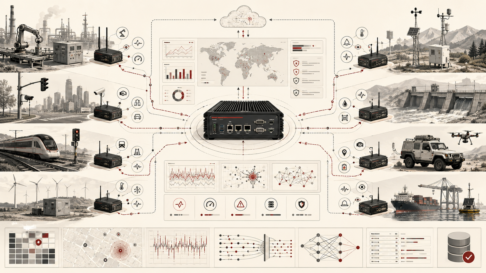
Distributed monitoring systems examine how multiple sensing, observation, or telemetry nodes work together to provide coordinated visibility into environmental, industrial, infrastructural, and operational conditions across time and space. In embedded and edge systems, distributed monitoring is not simply the deployment of many sensors. It is the architectural problem of turning local measurements into coherent system awareness through topology, timing discipline, communications, buffering, calibration, quality flags, supervision, aggregation, fault containment, and disciplined interpretation.
Many real-world systems cannot be understood from a single measurement point. Water quality changes along channels and catchments. Air conditions vary across streets, rooms, facilities, and neighborhoods. Industrial plants contain multiple failure surfaces rather than one. Buildings, utility assets, logistics networks, ecological sites, transportation corridors, and distributed infrastructure all generate conditions that are geographically and functionally dispersed. A single node can measure locally, but it cannot represent the full system unless it is placed within a wider monitoring architecture.
A distributed monitoring system therefore combines embedded devices, communications paths, time synchronization, power management, local storage, gateway logic, edge processing, data-quality controls, observability, and operational workflows. Each node may be simple, but the system as a whole is not. Once measurements are distributed, engineers must decide how nodes are synchronized, how missing data are handled, how partial failure is detected, how faults are localized, how measurements are compared across devices, and how system operators distinguish a meaningful event from network noise, stale telemetry, backfilled data, degraded visibility, or a failed observation path.
The most important shift is conceptual. A distributed monitoring system does not merely collect many local readings. It constructs a shared observational field in which each node contributes partial evidence to a larger representation of conditions. Whether that representation is trustworthy depends on the integrity of the whole chain: sensing, timing, transport, buffering, calibration, aggregation, supervision, fault containment, and interpretation.
Main Library
Publications
Article Map
Embedded & Edge Systems
Related Topic
Data Systems & Analytics
Related Topic
Environmental Monitoring
Related Topic
Intelligent Infrastructure
For engineers, the central question is not whether many devices can produce many readings. The question is whether those readings can be made comparable, timely, qualified, spatially meaningful, and operationally useful as evidence about a larger system. A distributed monitoring architecture must preserve node identity, location context, event time, freshness, quality state, calibration status, transport provenance, gateway behavior, aggregation lineage, and fault visibility. Without those controls, the system may appear richly instrumented while providing weak situational awareness.
Engineering Problem
The engineering problem is how to convert many local measurements into trustworthy system-level awareness. A distributed monitoring system must determine not only what each node measured, but where it measured, when it measured, how fresh the measurement is, how reliable the node is, how the measurement moved, whether data were delayed or backfilled, what quality state qualified the value, and whether the overall network still provides enough coverage to support the intended decision.
This problem becomes difficult because distributed monitoring systems fail partially more often than completely. One node may drift. Another may lose power. A gateway may buffer data during an outage. A cluster may go silent. A time source may degrade. A mesh route may change. A sensor may remain online while producing low-quality measurements. A dashboard may show recent values from some locations and stale values from others. These are not edge cases; they are normal conditions in fielded systems.
Weak distributed monitoring architectures treat the network as a collection of independent data sources. Strong architectures treat the network as a coordinated evidence system. They preserve node identity, spatial context, event time, freshness, calibration state, uncertainty, quality flags, connectivity state, queue state, gateway transformation history, aggregation lineage, and coverage state. This allows engineers to distinguish system conditions from monitoring-system conditions: a real environmental change from a missing node, a true industrial anomaly from a gateway delay, or a quiet process from a loss of visibility.
The practical engineering question is therefore: can the architecture produce coherent system awareness even when nodes drift, links fail, clocks slip, buffers fill, data arrive late, and parts of the monitoring network degrade?
Reference Architecture
A practical distributed monitoring architecture separates responsibilities across sensing nodes, local acquisition, timing, communications, gateways, edge coordination, ingestion, storage, analytics, observability, and operations. These layers may be physically combined in small systems, but the responsibilities still need to be explicit.
| Layer | Engineering Role | Integrity Risk | Evidence Artifact |
|---|---|---|---|
| Physical observation field | Defines the real-world system, geography, process, asset, or environment being monitored | Ambiguous monitoring objective, poor coverage assumptions | Monitoring objective, site map, process model, coverage plan |
| Monitoring nodes | Acquire local measurements, timestamps, health state, and quality indicators | Node drift, power loss, missing quality flags, weak local state | Node inventory, firmware version, calibration status, health heartbeat |
| Topology and placement | Determines spatial coverage, redundancy, reference nodes, and monitoring geometry | Coverage gaps, false representativeness, weak anomaly localization | Topology map, node role manifest, coverage model |
| Time discipline | Aligns measurements across nodes and preserves event-time semantics | False comparability, stale state, poor incident reconstruction | Clock status, synchronization method, drift estimate, timestamp fields |
| Communications layer | Moves data through wired, wireless, mesh, LPWAN, cellular, or gateway-mediated paths | Delay, packet loss, duplicate replay, hidden drops | Transport log, sequence number, retry count, delivery metadata |
| Gateway layer | Aggregates, buffers, translates, supervises, and coordinates local nodes | Opaque transformation, single point of local failure, lost lineage | Gateway manifest, buffer ledger, transformation version, child-node status |
| Edge coordination layer | Runs local rules, event detection, summarization, and site-level logic | Hidden inference, stale local policy, unqualified local alerts | Rule version, model version, local decision log, authority boundary |
| Ingestion and storage layer | Validates schema, preserves records, supports replay, and routes data | Schema drift, duplicate ingestion, timestamp collapse, quality loss | Data contract, schema version, idempotency key, ingestion result |
| Aggregation and interpretation layer | Turns local evidence into system-level indicators, maps, alerts, or diagnostics | Overconfident fusion, poor weighting, loss of raw evidence | Aggregation manifest, confidence weighting, lineage record |
| Observability and operations layer | Tracks monitoring-system health, gaps, freshness, coverage, and incidents | System appears healthy while observation capacity degrades | Monitoring health dashboard, fault log, coverage status, incident record |
This architecture makes distributed monitoring legible. It prevents engineers from treating system visibility as a simple consequence of node count and forces attention to the evidence chain that makes many local measurements meaningful together.
Implementation Pattern
A rigorous distributed monitoring implementation begins by defining the monitoring objective, node roles, topology, timing discipline, communications path, buffering policy, quality policy, aggregation method, observability signals, and incident-reconstruction requirements. The system should specify not only how data are collected, but how they remain comparable, fresh, qualified, and interpretable across the monitoring field.
| Artifact | Purpose | Typical Format |
|---|---|---|
| Monitoring objective | Defines whether the system supports early warning, trend analysis, diagnostics, compliance, control, or situational awareness | Markdown, YAML, engineering specification |
| Node inventory | Maps node ID, role, location, sensor type, firmware, calibration, power state, and owner | CSV, SQL, JSON |
| Topology map | Defines node placement, coverage zones, reference nodes, gateways, and monitoring geometry | GeoJSON, CSV, GIS layer, graph file |
| Timing policy | Defines synchronization method, timestamp fields, clock-drift limits, and allowed temporal skew | YAML, firmware config, data contract |
| Transport policy | Defines communication path, retry behavior, sequence numbers, delivery guarantees, and drop semantics | YAML, protocol config, broker policy |
| Buffering and backfill policy | Defines local storage, queue depth, replay ordering, idempotency, and late-arrival handling | YAML, firmware config, gateway config |
| Quality policy | Defines calibration status, uncertainty, confidence, node authority, quality flags, and validation rules | YAML, JSON Schema, SQL |
| Fault-containment policy | Defines which node, gateway, clock, quality, and coverage faults block specific downstream uses | YAML, state machine, operational rule set |
| Gateway transformation manifest | Documents translation, filtering, aggregation, unit conversion, and lineage preservation | YAML, code manifest, edge rule config |
| Aggregation manifest | Defines weighting, fusion, interpolation, anomaly logic, summary rules, and confidence propagation | YAML, notebook, analytics config |
| Monitoring observability schema | Defines health signals for node liveness, freshness, coverage, queue pressure, drift, fault state, and gaps | JSON Schema, metrics registry, SQL |
| Incident reconstruction policy | Defines which evidence must exist to explain system events, outages, and monitoring gaps | Markdown, YAML, audit log specification |
The implementation goal is to make distributed visibility auditable. Engineers should be able to reconstruct not only what the monitored system was doing, but what the monitoring network could actually see at the time.
Formal Model: Distributed Monitoring as Coordinated Evidence
Distributed monitoring can be modeled as a set of local observations that are transformed into a system-level state estimate. Let \(x(s,t)\) represent the condition of interest at location or system position \(s\) and time \(t\). Each node \(i\) observes only part of that field.
y_i(t) = h_i(x(s_i,t)) + n_i(t) + b_i(t)
\]
Interpretation: Node \(i\) observes the condition at location \(s_i\) through measurement function \(h_i\), noise \(n_i(t)\), and bias or drift \(b_i(t)\). Distributed monitoring must account for node-specific error rather than assuming all observations are equally authoritative.
\hat{x}(s,t) = F(y_1,\ldots,y_N,\tau_1,\ldots,\tau_N,q_1,\ldots,q_N)
\]
Interpretation: A system-level estimate depends on node measurements \(y_i\), timestamp states \(\tau_i\), and quality states \(q_i\). Aggregation is only trustworthy if time and quality information are preserved.
F_{\mathrm{fresh},i} = t_{\mathrm{now}} – t_{\mathrm{event},i}
\]
Interpretation: Freshness is measured from event time, not arrival time. A delayed but successfully delivered record may be useful historically while being unsuitable for real-time monitoring.
\Delta t_{ij} = |t_i – t_j|
\]
Interpretation: Cross-node temporal skew \(\Delta t_{ij}\) determines whether measurements from nodes \(i\) and \(j\) can be compared as representing the same event or time window.
C_{\mathrm{coverage}} = \frac{A_{\mathrm{observed}}}{A_{\mathrm{required}}}
\]
Interpretation: Coverage completeness compares the portion of the required monitoring field currently observed to the portion that must be observed for the system’s intended use.
H_{\mathrm{monitor}} = w_1 L_{\mathrm{node}} + w_2 F_{\mathrm{fresh}} + w_3 C_{\mathrm{coverage}} + w_4 Q_{\mathrm{data}} + w_5 S_{\mathrm{sync}} + w_6 G_{\mathrm{gateway}}
\]
Interpretation: Monitoring health can combine node liveness, freshness, coverage, data quality, synchronization status, and gateway health into a practical operational score.
These formulas do not replace engineering judgment. They make explicit that distributed monitoring quality depends on more than data volume. It depends on coverage, timing, freshness, quality, synchronization, and visibility into the monitoring system itself.
Monitoring State Model
A distributed monitoring system should expose its own state clearly. Without a monitoring-state model, dashboards often collapse distinct conditions into the same visual result. A quiet process, a stale node, a failed gateway, a delayed backfill, a low-quality reading, and a complete coverage loss may all appear as “normal” unless the architecture preserves state explicitly.
| Monitoring State | Meaning | Allowed Interpretation | Required Action |
|---|---|---|---|
observed_valid |
Required node or zone is reporting fresh, synchronized, quality-qualified data | Eligible for normal monitoring, aggregation, alerts, and dashboards | Continue normal operation |
observed_low_confidence |
Data are present but affected by quality, calibration, noise, or uncertainty concerns | Use only with confidence qualification | Surface quality warning and investigate cause |
observed_stale |
Data are present but older than the operational freshness requirement | Historical use only; not current state | Mark stale and block real-time use |
coverage_degraded |
Some required zones or node roles are missing or below threshold | System-level conclusions should be qualified | Show coverage gap and maintenance priority |
gateway_degraded |
Gateway is delaying, buffering, dropping, or losing child-node visibility | Local cluster visibility is weakened | Inspect gateway, transport, and buffer state |
sync_degraded |
Clock drift or timestamp uncertainty exceeds the use-case threshold | Temporal comparisons and event propagation analysis are restricted | Resynchronize or exclude from time-sensitive fusion |
backfill_replay |
Delayed records are being uploaded after outage or buffering | Useful for historical reconstruction, not live state | Use event-time ordering and idempotency controls |
visibility_lost |
Required monitoring region, node group, or gateway cluster is not observable | No valid conclusion about current state | Escalate as observation-system failure |
This state model protects interpretation. It prevents the system from presenting all numeric values as equally current, all gaps as equally harmless, and all summaries as equally authoritative. The monitoring state should travel with the measurement, the map, the dashboard, and the aggregated indicator.
What Are Distributed Monitoring Systems?
Distributed monitoring systems are architectures in which multiple devices, sensing points, or observation nodes measure different parts of a system, environment, or operational field and contribute those measurements to a broader monitoring model. Each device produces local data, but the monitoring system only becomes useful when those local observations are made comparable, transportable, qualified, and interpretable at the system level.
What distinguishes distributed monitoring from simple data collection is coordination. The system must define relationships among nodes, timing behavior, reporting paths, quality states, topology, aggregation logic, and supervision. A distributed monitoring system is not just an inventory of devices. It is a structured observational system with rules for how evidence is generated, moved, validated, fused, and interpreted.
In practical terms, distributed monitoring systems can be centralized, hierarchical, peer-assisted, edge-coordinated, or hybrid. Some push all data toward a central repository. Others rely on gateways or local hubs. Some allow nodes or edge tiers to perform local interpretation before forwarding summaries or anomalies. The architecture depends on the monitoring problem: environmental sensing, asset health, industrial telemetry, building systems, power infrastructure, transport networks, water systems, agriculture, logistics, or site-scale edge operations.
The main challenge is that distributed monitoring can create a convincing appearance of visibility without actually producing coherent awareness. A map full of sensors may still be weak if the nodes are badly placed, poorly synchronized, unevenly calibrated, intermittently connected, or unable to expose their own health state. The architecture must therefore make visibility itself measurable.
Monitoring Nodes as Embedded Observation Points
Each node in a distributed monitoring system is an embedded observation point. It is responsible for sensing, local timing, limited storage, communications behavior, and enough self-supervision to remain a trustworthy participant in the broader system. Even when nodes are simple, they are not passive. They embody assumptions about what is worth measuring, how often it should be measured, how values are timestamped, how data are buffered, and under what operating conditions the node can be trusted.
This is why node architecture matters. A network of weak nodes does not become strong merely by multiplication. If local sensing is unstable, if power fails unpredictably, if clocks drift too far, if firmware does not preserve state during outages, or if node health is invisible, aggregation will amplify uncertainty rather than resolve it. Distributed monitoring begins with dependable local observation, not with dashboard design.
| Node Responsibility | Engineering Requirement | Failure Risk | Evidence to Preserve |
|---|---|---|---|
| Local sensing | Measure defined variables within calibrated range | Invalid local values become part of system-level interpretation | Sensor ID, calibration status, measurement range, quality flag |
| Timestamping | Record event time and clock status | Cross-node comparison becomes misleading | Event time, clock source, drift estimate, synchronization state |
| Local buffering | Preserve data through short outages | Silent data loss or ambiguous backfill | Queue depth, sequence number, replay batch, drop reason |
| Power management | Maintain predictable sampling and reporting under power limits | Intermittent operation mistaken for environmental silence | Battery state, duty cycle, expected reporting interval |
| Self-supervision | Report health, faults, reset events, and degraded states | Node appears normal while its observation quality declines | Heartbeat, reset count, fault code, degraded-mode flag |
| Identity and role | Expose node identity, location, and monitoring role | Data cannot be placed correctly in system context | Node ID, role, location, firmware version, configuration version |
Node design also depends on role. Some nodes are fixed and persistent, others mobile, intermittent, or opportunistic. Some are dense low-cost devices intended to increase spatial coverage. Others are fewer but higher-assurance reference points. The value of the system often depends on how these different node types are combined and whether their differing reliability, authority, and uncertainty are made explicit in downstream interpretation.
Topology, Coverage, and Monitoring Geometry
Distributed monitoring systems are shaped by topology: where nodes are placed, how densely they are deployed, what they can actually observe, and how their observation zones overlap. Coverage is never purely quantitative. Ten badly placed nodes may produce less useful system awareness than three well-sited nodes that align with the structure of the monitored process.
Monitoring geometry is therefore an architectural concern. A distributed system should make clear whether it is designed to detect gradients, coverage gaps, anomalies, boundary conditions, process transitions, spatial correlations, propagation patterns, or representative baseline conditions. Different goals produce different placement logic. A system designed for early warning has different topology needs than one designed for long-term trend analysis or localized diagnostics.
| Monitoring Goal | Topology Implication | Engineering Risk |
|---|---|---|
| Early warning | Place nodes near likely sources, boundaries, or leading indicators | Event detected too late or only after propagation |
| Gradient detection | Place nodes across expected spatial or process gradients | System misses direction, intensity, or spread |
| Coverage assurance | Ensure required zones remain observed even under node failure | Blind spots hidden by overall node count |
| Reference validation | Use higher-assurance nodes to anchor lower-cost nodes | Low-cost drift becomes invisible |
| Anomaly localization | Use enough spatial resolution and overlap to isolate source | Alerts cannot distinguish local fault from system event |
| Trend analysis | Prioritize stable, consistent, long-lived monitoring locations | Topology changes masquerade as environmental or process changes |
Good distributed monitoring design therefore treats node placement as part of system modeling. It asks what relationships among locations matter and what kinds of inference the network should and should not support. A topology that looks visually comprehensive may still be analytically weak if node locations do not align with the actual structure of the monitored process.
Coverage and Inference Boundaries
A distributed monitoring network does not observe everything equally. Every topology creates inference boundaries: places, times, or operating states where the system can support a conclusion, and places where it cannot. A technically mature monitoring architecture makes those boundaries visible instead of implying that instrumentation equals total awareness.
This matters because downstream users often treat maps, dashboards, and aggregate indicators as complete representations. But every system-level claim depends on coverage, node authority, spatial density, synchronization, freshness, and quality. A monitoring network can support “conditions at this node,” “conditions in this zone,” “a likely gradient between these points,” or “system-level state with degraded confidence.” Those are different claims.
| Claim Type | Required Evidence | Unsupported When… |
|---|---|---|
| Node-local condition | Fresh, calibrated, quality-valid measurement from a known node | Node is stale, low-quality, uncalibrated, or missing |
| Zone condition | Required node coverage within the zone and valid aggregation rule | Coverage falls below threshold or node roles are incomplete |
| Cross-node comparison | Comparable calibration, synchronized event times, and compatible measurement semantics | Clock skew, sensor mismatch, or quality asymmetry exceed thresholds |
| Gradient or spatial trend | Node placement across expected gradient and sufficient spatial density | Topology does not sample the gradient path |
| Event propagation | Strong timing discipline and known node positions | Event times are delayed, backfilled, or unsynchronized |
| System-level health | Coverage, freshness, quality, and aggregation confidence preserved | Partial visibility is hidden or aggregation lineage is missing |
Inference boundaries are not a weakness. They are a sign of engineering honesty. A monitoring system that states what it cannot currently know is more trustworthy than one that fills every dashboard cell with unqualified certainty.
Time Synchronization and Cross-Node Comparability
Once many nodes are measuring at once, time becomes one of the most important system properties. Measurements that appear comparable may not describe the same moment or the same event unless clocks are aligned closely enough for the intended use. A distributed monitoring system therefore needs explicit time discipline, whether through real-time clocks, gateway correction, network time protocols, GPS timing, bounded drift assumptions, or event-based alignment.
The tighter the interpretive coupling among nodes, the more important synchronization becomes. Systems that collect slow-moving background conditions can tolerate looser time coherence. Systems that compare flows, event propagation, vibration, synchronized control conditions, or transient anomalies often cannot. Timing is therefore part of what gives a distributed monitoring system epistemic integrity.
| Timing Concern | Engineering Question | Failure Mode | Control Pattern |
|---|---|---|---|
| Clock drift | How far can a node clock move between synchronization events? | Measurements appear aligned but are not | Drift bounds, periodic sync, clock-health metadata |
| Event time | When did the physical measurement occur? | Arrival time mistaken for acquisition time | Preserve event time separately from ingestion time |
| Gateway receive time | When did an intermediate layer receive the record? | Local transport delay becomes invisible | Gateway timestamp, upload timestamp, replay batch |
| Cross-node skew | Are two nodes close enough in time to compare? | False causality or false correlation | Temporal windows and skew thresholds by use case |
| Backfill timing | Were records delayed and uploaded later? | Historical data mistaken for live state | Replay flags, event-time ordering, idempotency keys |
| Processing time | When did analytics or rules use the record? | Incident reconstruction cannot explain decisions | Processing timestamp, rule version, decision log |
Time also creates hierarchy. There is the local sampling time at the node, the transport time across the network, the gateway time, and the ingestion time at the aggregation layer. Mature systems preserve all of these when they matter, because collapsing them into one timestamp can make late-arriving data look fresh or make synchronized data look asynchronous.
Communications, Gateways, and Data Transport
Distributed monitoring systems must move data from nodes to places where those data can be fused, reviewed, or acted upon. This can happen through direct cellular links, wired plant networks, short-range radio, LPWAN, mesh relay, fieldbus systems, industrial gateways, or intermediary edge nodes. The choice is not only about convenience or bandwidth. It shapes fault behavior, latency, power use, autonomy, security exposure, and how much operational state field nodes must sustain.
Gateway architectures often occupy a useful middle ground. They reduce per-node communications burden, enable local coordination, and can perform buffering, supervision, or translation before pushing data onward. But gateways also create concentration points. A gateway failure can isolate many healthy nodes at once. Direct-to-cloud models remove that dependency but may increase per-node complexity and energy cost.
| Transport Pattern | Strength | Risk | Required Evidence |
|---|---|---|---|
| Direct-to-cloud | Simple upstream path, fewer local infrastructure dependencies | Higher endpoint power and complexity, weak local resilience | Device identity, retry log, delivery metadata, connectivity state |
| Gateway-mediated | Local aggregation, buffering, translation, and supervision | Gateway becomes local concentration point | Gateway health, child-node status, buffer ledger, transformation manifest |
| Mesh relay | Extends coverage and supports peer-assisted transport | Routing complexity, variable latency, hard-to-debug packet paths | Route state, hop count, link quality, delay metadata |
| LPWAN | Long-range, low-power telemetry | Limited bandwidth, delayed reporting, sparse payloads | Payload schema, duty-cycle policy, freshness rules |
| Wired industrial network | Stable, deterministic, integration with existing assets | Legacy protocol translation and boundary risk | Protocol map, gateway rule version, unit normalization |
| Store-and-forward | Improves continuity during outages | Replay ambiguity and duplicate ingestion | Event time, replay batch, idempotency key, sequence number |
The communications path belongs inside the monitoring model itself. A system that cannot explain how data move, how delays occur, and what happens under loss of connectivity is not only weak operationally; it is also weaker interpretively because users cannot distinguish a quiet system from an unseen one.
Buffering, Backfill, and Intermittent Connectivity
Real distributed monitoring systems rarely enjoy perfect connectivity. Nodes may sleep, links may drop, gateways may restart, and uplinks may become intermittent. For that reason, buffering is not merely a convenience. It is part of the architecture of continuity. Nodes and gateways need enough storage and sequencing logic to preserve useful history until transport resumes, and the system needs a backfill model that makes late-arriving data coherent rather than confusing.
Backfill raises interpretive questions as well as operational ones. A measurement received now may describe a condition from minutes or hours ago. That is acceptable only if the system preserves timestamp integrity and clearly distinguishes acquisition time from ingestion time. This is another reason distributed monitoring systems should retain provenance rather than collapse all events into one undifferentiated stream.
| Buffering Question | Engineering Decision | Risk if Undefined |
|---|---|---|
| What gets buffered? | Raw readings, quality-qualified records, alarms, summaries, or priority classes | Critical evidence lost while low-value data are retained |
| How long is data retained? | Time limit, record limit, or priority-dependent retention | Old records silently displace useful evidence |
| What is dropped under pressure? | Drop policy by priority, age, or data class | Silent loss and false completeness |
| How is replay ordered? | Event time, sequence number, priority, or upload order | Backfilled data distort trends and event sequences |
| How are duplicates prevented? | Idempotency key, sequence number, replay window | Analytics double-count delayed records |
| How is stale data marked? | Freshness threshold, backfill flag, quality state | Historical data presented as live state |
A mature system treats intermittent connectivity as expected behavior. It specifies what is buffered, how long it can be retained, how ordering is preserved, and what happens when local storage fills or transport is delayed beyond acceptable use. Buffer policy is part of the monitoring design, not just a firmware implementation detail.
Freshness, Latency, and Monitoring Semantics
One of the most common weaknesses in distributed monitoring is the failure to distinguish freshness from simple data presence. A dashboard may show a value, but that does not mean the value is recent enough to support the decision being made. A system can therefore appear operational while actually presenting stale observations.
Freshness should be modeled explicitly. Each measurement has a recency window within which it remains meaningful for a given use case. That window may be seconds for control-relevant telemetry, minutes for anomaly awareness, or hours for slower environmental trends. Once that window is exceeded, the data may still be historically useful but no longer operationally current.
| Use Case | Freshness Requirement | Interpretive Risk | Required System Behavior |
|---|---|---|---|
| Real-time alarm | Seconds to short minutes | Delayed event appears current | Reject stale data from alarm generation |
| Operational dashboard | Seconds to minutes depending on process | Operators act on old state | Display age and quality state visibly |
| Trend analysis | Minutes to hours depending on domain | Backfill may distort time series if ordered incorrectly | Use event-time ordering and replay metadata |
| Compliance reporting | Completeness and provenance may matter more than immediacy | Missing or low-quality records treated as valid evidence | Preserve gaps, quality flags, and calibration state |
| Edge control | Strict freshness and deterministic behavior | Unsafe action based on stale state | Local freshness gate and fail-safe behavior |
Latency semantics matter just as much. Some monitoring architectures optimize for immediate visibility, others for eventual completeness, and others for a balance between the two. The system should make clear whether users are viewing live state, delayed state, backfilled history, or fused summaries that incorporate both recent and older inputs. Without that clarity, system awareness becomes visually persuasive but temporally ambiguous.
Data Quality, Calibration, and Cross-Node Validation
Distributed monitoring systems are only as trustworthy as their ability to compare measurements across nodes without pretending all nodes are equally valid at all times. Calibration drift, environmental exposure, local noise, sensor aging, maintenance asymmetry, and installation differences all create cross-node inconsistency.
Cross-node validation can take several forms: collocation with reference nodes, overlapping monitoring zones, sanity checks across neighboring devices, calibration metadata, maintenance histories, redundant measurement paths, and data-quality flags that persist into downstream analysis. These mechanisms matter because a distributed system should not silently assume that every node remains equally reliable over time.
| Quality Mechanism | Purpose | Engineering Benefit |
|---|---|---|
| Reference node | Provides higher-assurance anchor for nearby nodes | Detects drift in lower-cost or field-exposed sensors |
| Collocation check | Compares nodes under shared conditions | Estimates bias and cross-node agreement |
| Neighbor consistency | Checks whether nearby nodes behave plausibly relative to each other | Detects isolated node faults or local anomalies |
| Calibration metadata | Preserves calibration status and coefficient version | Prevents expired or uncalibrated values from being treated as valid |
| Uncertainty propagation | Carries measurement confidence into aggregation | Prevents overconfident system-level summaries |
| Quality flags | Marks stale, low-confidence, inferred, saturated, or suspect records | Allows downstream systems to qualify use |
A strong monitoring architecture includes not only data transport, but quality transport. Uncertainty, calibration state, maintenance status, and detected anomalies should travel with the measurements they qualify. In a mature system, a node’s authority is contextual rather than assumed.
Fault Visibility, Partial Failure, and System Supervision
Distributed monitoring systems fail partially more often than completely. One node drifts, another loses power, a gateway stalls, a radio path weakens, a storage queue backs up, or a cluster of devices becomes unavailable. These partial failures are especially dangerous when the system continues to appear healthy from a central viewpoint.
This is why distributed supervision must include node liveness, freshness of reporting, gap detection, reset visibility, queue state, gateway health, synchronization status, and enough internal status to distinguish missing data from quiet conditions. In a fielded monitoring system, “no change” and “no visibility” are not the same state.
| Failure Condition | How It Appears | How It Should Be Detected | Operational Response |
|---|---|---|---|
| Node offline | No recent readings | Heartbeat age, expected reporting interval, connectivity state | Mark coverage gap and alert maintenance |
| Node drift | Values gradually diverge from nearby/reference nodes | Cross-node validation, calibration trend, residual analysis | Reduce confidence and schedule recalibration |
| Gateway outage | Many child nodes disappear together | Gateway heartbeat, child-node reporting collapse, buffer state | Switch local mode and mark site visibility degraded |
| Queue pressure | Data delayed or dropped | Queue depth, buffer pressure, drop reason | Adjust reporting, prioritize records, investigate transport |
| Clock drift | Cross-node comparisons become inconsistent | Clock-health status, drift estimate, sync age | Exclude from time-sensitive fusion until resynchronized |
| Silent data loss | Dashboard appears sparse but not failed | Sequence gaps, expected-count checks, delivery ratio | Surface completeness warning and reconstruct gaps |
Partial-failure awareness also affects recovery design. Some faults should be handled locally through retry, peripheral reset, local buffering, or degraded mode. Others should be escalated to gateways or operators. The monitoring system should not only detect faults in what it measures; it should detect faults in its own ability to measure.
Fault Containment and Quality Gating
Distributed monitoring systems need fault containment because weak observations can contaminate system-level interpretation. A stale node should not drive a real-time alert. A low-confidence node should not carry the same aggregation weight as a calibrated reference node. A gateway replay should not be mistaken for live state. A time-unsynchronized cluster should not be used for event-propagation analysis. Quality gating turns these distinctions into enforceable rules.
| Condition | Allowed Use | Restricted Use | Containment Action |
|---|---|---|---|
valid_fresh_synchronized |
Normal aggregation, alerts, dashboards, and operational reporting | None under normal requirements | Continue monitoring |
stale |
Historical reconstruction and trend backfill | Real-time alerting, live dashboard state, control decisions | Mark stale and block operational use |
low_confidence |
Qualified trend context and diagnostic review | High-confidence aggregation or compliance evidence without qualification | Reduce weight and surface quality warning |
sync_degraded |
Slow-moving trend analysis if timing tolerance permits | Propagation analysis, transient correlation, synchronized fusion | Exclude from time-sensitive aggregation |
coverage_degraded |
Local conclusions in observed zones | System-wide claims or full-field maps without qualification | Display coverage gap and confidence boundary |
gateway_replay |
Historical recovery and completeness repair | Live status or immediate alarm generation | Use event-time ordering and idempotency checks |
node_drift_warning |
Diagnostic comparison and provisional monitoring | Unweighted aggregation or high-trust reference use | Reduce authority and schedule recalibration |
visibility_lost |
None for current-state claims in affected zone | All current monitoring conclusions for affected zone | Escalate as monitoring-system fault |
Fault containment prevents a monitoring-system failure from becoming a false claim about the monitored system. The goal is not to discard every imperfect record. The goal is to prevent each record from being used beyond the evidence it can support.
Aggregation, Fusion, and System-Level Interpretation
Aggregation is the point at which local observations become system awareness. But aggregation is not just averaging. It may involve temporal alignment, spatial interpolation, threshold logic, anomaly detection, cross-sensor consistency checks, confidence weighting, graph-based propagation, or multi-level summaries that distinguish raw signals from derived indicators.
The more distributed the system becomes, the more important it is to preserve the distinction between observation and inference. A derived state estimate is only useful if the system can explain which underlying measurements contributed to it, under what timing assumptions, and with what quality or confidence state.
| Aggregation Pattern | Use | Integrity Requirement |
|---|---|---|
| Simple averaging | Stable, comparable nodes measuring similar quantities | Comparable calibration, timing window, and quality state |
| Confidence-weighted fusion | Nodes have different uncertainty, quality, or authority | Preserved uncertainty and quality flags |
| Spatial interpolation | Estimating conditions between nodes | Topology awareness, coverage limits, uncertainty bands |
| Temporal alignment | Comparing events across nodes | Event time, synchronization state, allowable skew |
| Anomaly detection | Identifying unusual system behavior | Separation of node fault from real system anomaly |
| Hierarchical summaries | Site, region, asset, or system-level dashboards | Lineage from summary back to source nodes |
Strong aggregation systems expose layers rather than flattening them. They retain access to node data, gateway-transformed data, and higher-level synthesized views. This makes the monitoring system more interpretable under both normal operation and anomaly investigation.
Edge Coordination and Local Intelligence
Distributed monitoring systems increasingly use local intelligence to reduce bandwidth, improve responsiveness, and support partial autonomy. Nodes or gateways may filter noise, detect threshold crossings, batch events, compress telemetry, perform local fusion, classify sensor states, or trigger local alerts before sending summaries onward. This can be beneficial, especially when communications are costly or unreliable.
But local intelligence changes governance. It shifts some interpretive authority away from the center and into field devices or intermediate gateways. That can improve responsiveness, but it also creates a stronger need for transparency around what was measured directly, what was filtered, what was inferred locally, what rules were active, and whether raw evidence remains available for reconstruction.
| Edge Function | Benefit | Risk | Evidence to Preserve |
|---|---|---|---|
| Local thresholding | Fast response and lower upstream traffic | Stale or incorrect thresholds create missed alerts | Rule version, threshold value, event log |
| Local filtering | Reduces noise and bandwidth | Suppresses transients or hides sensor faults | Filter version, raw-retention policy, quality state |
| Gateway fusion | Creates site-level summaries | Loss of node-level evidence | Fusion manifest, contributing nodes, confidence weights |
| TinyML classification | Supports local event detection under bandwidth limits | Model drift or opaque confidence | Model version, confidence, fallback behavior |
| Local degraded mode | Maintains site awareness during outage | Local state may diverge from central state | Offline-mode policy, local decision log, replay record |
Good distributed monitoring design treats edge processing as a formal layer in the system rather than a hidden optimization. The system should preserve enough lineage that local decisions do not make central interpretation more opaque, and enough policy clarity that local actions remain aligned with the larger monitoring objective.
Fleet Observability and Monitoring Health
A distributed monitoring system must observe itself. A system that reports only measured values cannot distinguish monitored-system silence from monitoring-system failure. Fleet observability therefore needs signals about node health, gateway health, clock health, queue depth, reporting gaps, data freshness, calibration status, quality state, coverage, and aggregation confidence.
| Operational Signal | What It Reveals | Why Engineers Need It |
|---|---|---|
| Node heartbeat age | How long since each node reported health | Detects silent node failure |
| Telemetry freshness | Age of measurements relative to event time | Separates live monitoring from delayed history |
| Coverage completeness | Share of required monitoring field currently observed | Surfaces blind spots and degraded system awareness |
| Clock synchronization status | Whether nodes remain comparable in time | Protects temporal analysis and event correlation |
| Queue depth | Buffer pressure at nodes or gateways | Detects transport bottlenecks before data loss |
| Sequence gaps | Missing or dropped records | Reveals incomplete data streams |
| Calibration status | Whether node measurements remain qualified | Prevents drift from contaminating aggregation |
| Gateway child-node reporting rate | Whether gateways still see their local fleet | Detects local cluster failure |
| Quality-state distribution | Share of valid, stale, low-confidence, inferred, or suspect records | Shows whether monitoring quality is degrading |
| Aggregation confidence | Confidence attached to system-level summaries | Prevents overconfident dashboards during partial visibility |
Monitoring observability should be designed before deployment. If the system cannot observe its own capacity to observe, then dashboards can become misleading exactly when they are most needed.
Worked Example: Distributed Water, Air, and Industrial Monitoring
Consider a mixed distributed monitoring deployment that spans a water-quality corridor, nearby air-quality stations, and industrial equipment nodes at several facilities. Some nodes are high-assurance reference points. Others are lower-cost distributed sensors. Gateways buffer data during outages. Edge nodes run local threshold rules. A central platform aggregates readings into dashboards, alerts, and historical analysis.
| Scenario | Architectural Risk | Required Design Response |
|---|---|---|
| Water-quality node upstream reports a sudden anomaly | Downstream nodes may not be synchronized closely enough for propagation analysis | Use event time, clock status, and temporal skew thresholds |
| Air-quality cluster loses a gateway | Dashboard may show regional calm while local visibility is missing | Mark coverage degraded and expose child-node reporting collapse |
| Industrial vibration node drifts slowly | Aggregation may treat drift as asset condition change | Use reference comparison, residual analysis, and drift warning flags |
| Gateway backfills records after outage | Delayed records may trigger false live alerts | Use replay batch, event-time ordering, freshness gates, and idempotency keys |
| Lower-cost nodes disagree with reference node | System may either ignore true local variation or accept bad data | Apply node authority, confidence weighting, and cross-node validation |
| Edge gateway filters noisy records | Central system may lose evidence needed for audit | Preserve filter version, raw-retention policy, and transformation lineage |
This example shows why distributed monitoring is not just a network problem. It is a coordinated evidence problem. The system must preserve timing, topology, node authority, quality state, replay semantics, and aggregation lineage so that operators can tell whether a system-level signal reflects the monitored world or the monitoring network itself.
Deployment Readiness Gate
An engineering-grade distributed monitoring system should pass a deployment readiness gate before field rollout. The gate should verify that the monitoring network can preserve coverage, timing, freshness, quality, supervision, and incident reconstruction under realistic operating conditions.
| Readiness Check | Pass Condition | Why It Matters |
|---|---|---|
| Monitoring objective defined | System purpose, decision context, and freshness requirements documented | Prevents vague visibility goals |
| Topology reviewed | Node placement, coverage zones, reference nodes, and gaps documented | Protects spatial validity |
| Inference boundaries documented | Supported and unsupported claims are stated by zone, timing, and quality state | Prevents overconfident system-level conclusions |
| Node inventory complete | Node ID, role, location, firmware, calibration, power, and owner recorded | Prevents unmanaged observation points |
| Timing policy validated | Clock source, drift limit, sync method, and timestamp fields verified | Protects cross-node comparability |
| Transport path tested | Retry, sequence, delivery, drop, and transport-delay behavior tested | Prevents silent data loss and ambiguous delivery |
| Buffering and replay tested | Queue limits, backfill, idempotency, freshness flags, and drop reasons verified | Prevents outage ambiguity |
| Quality policy implemented | Calibration, uncertainty, quality flags, and node authority are preserved | Prevents weak records from becoming authoritative |
| Fault containment implemented | Stale, low-confidence, unsynchronized, replayed, and coverage-degraded states gate downstream use | Prevents monitoring faults from becoming false system claims |
| Gateway behavior documented | Transformations, filtering, aggregation, buffering, and child-node status are visible | Prevents semantic loss at boundary layers |
| Aggregation lineage preserved | System-level indicators can be traced to source nodes and assumptions | Supports debugging and audit |
| Monitoring observability implemented | Freshness, liveness, coverage, queue pressure, clock status, and quality state visible | Allows engineers to operate the monitoring system |
| Incident reconstruction ready | Evidence can reconstruct node, gateway, transport, ingestion, and aggregation behavior | Supports accountability after failure or anomaly |
This readiness gate separates a collection of deployed sensors from a fieldable distributed monitoring architecture.
Data and Configuration Artifacts
Distributed monitoring becomes easier to operate when assumptions are represented as machine-readable artifacts. These artifacts allow engineers to validate coverage, timing, quality, replay, aggregation, gateway behavior, and monitoring health rather than relying on informal diagrams or undocumented operational knowledge.
| Artifact | What It Captures | Engineering Purpose |
|---|---|---|
node_inventory.csv |
Node identity, role, location, firmware, calibration, power, owner, and status | Creates a fleet-level view of monitoring assets |
topology_map.geojson |
Node placement, coverage zones, gateways, and monitored field boundaries | Supports coverage and spatial reasoning |
timing_policy.yml |
Clock source, drift limits, timestamp requirements, and skew thresholds | Protects cross-node comparability |
transport_policy.yml |
Protocol, retry, sequencing, delivery, and drop semantics | Makes communications behavior inspectable |
buffering_replay_policy.yml |
Queue depth, backfill, ordering, idempotency, and stale-data marking | Controls intermittent connectivity |
quality_policy.yml |
Calibration state, uncertainty, confidence, and quality flags | Preserves measurement fitness for use |
fault_containment_policy.yml |
Quality gates for stale, degraded, replayed, unsynchronized, and low-confidence records | Prevents weak records from driving unsupported decisions |
gateway_manifest.yml |
Gateway transformations, filtering, aggregation, and child-node supervision | Prevents hidden semantic changes |
aggregation_manifest.yml |
Fusion method, weighting, interpolation, anomaly logic, and lineage rules | Makes system-level interpretation auditable |
monitoring_health_schema.json |
Freshness, liveness, coverage, queue pressure, clock status, and quality signals | Supports fleet observability |
deployment_readiness.yml |
Pre-field checks for coverage, timing, transport, quality, observability, and reconstruction | Turns trustworthiness into a testable gate |
The goal is not documentation for its own sake. The goal is operational memory. When a distributed monitoring system is challenged, debugged, audited, or improved, the system should be able to reconstruct both the state of the monitored system and the state of the monitoring network that observed it.
Mathematical Lens: Coverage, Freshness, Synchronization, and Confidence
A practical mathematical lens for distributed monitoring focuses on whether the monitoring network can produce usable system awareness under partial visibility.
C_{\mathrm{coverage}} = \frac{N_{\mathrm{active\ required\ zones}}}{N_{\mathrm{required\ zones}}}
\]
Interpretation: Coverage completeness measures whether the required monitoring zones are currently represented by active, usable nodes.
R_{\mathrm{delivery}} = \frac{N_{\mathrm{received}}}{N_{\mathrm{expected}}}
\]
Interpretation: Delivery reliability compares received records to expected records. It should be interpreted alongside freshness and quality, not alone.
F_{\mathrm{fresh}} = t_{\mathrm{now}} – t_{\mathrm{event}}
\]
Interpretation: Freshness measures age relative to event time. A record can be delivered successfully and still be too old for operational use.
S_{\mathrm{sync}} = \max_{i,j} |t_i – t_j|
\]
Interpretation: Synchronization spread measures the maximum time difference across nodes being compared. It must be bounded for time-sensitive interpretation.
Q_{\mathrm{usable}} = \frac{N_{\mathrm{valid, fresh, synchronized}}}{N_{\mathrm{received}}}
\]
Interpretation: Usable monitoring rate measures the share of received records that are valid, fresh, and synchronized enough for the intended monitoring purpose.
B_{\mathrm{pressure}} = \frac{Q_{\mathrm{current}}}{Q_{\mathrm{capacity}}}
\]
Interpretation: Buffer pressure compares current queue depth to capacity. High pressure indicates outage, transport bottleneck, or ingestion failure.
M_{\mathrm{health}} = w_1 C_{\mathrm{coverage}} + w_2 Q_{\mathrm{usable}} + w_3 R_{\mathrm{delivery}} + w_4 S_{\mathrm{sync}} + w_5 H_{\mathrm{gateway}} + w_6 O_{\mathrm{observable}}
\]
Interpretation: Monitoring health can combine coverage, usable telemetry, delivery, synchronization, gateway health, and observability coverage into a practical operational index.
The purpose of these formulas is not to reduce distributed monitoring to a single score. It is to make key architectural properties measurable: coverage, freshness, delivery, synchronization, queue pressure, quality, and observability.
Python Workflow: Distributed Monitoring Health and Coverage Analysis
The companion Python workflow should model a distributed monitoring network across nodes, gateways, topology zones, telemetry records, freshness, timing skew, quality state, buffer pressure, coverage completeness, replay behavior, and inference boundaries. It can identify stale zones, missing nodes, gateway bottlenecks, duplicate replay, coverage gaps, clock-skew violations, and weak aggregation confidence.
# Python Workflow: Distributed Monitoring Health and Coverage Analysis

nodes["active"] = (
    (nodes["connectivity_state"] == "online")
    & (nodes["health_state"] == "healthy")
    & (nodes["calibration_state"] == "valid")
)

telemetry["freshness_seconds"] = (
    telemetry["processing_time"] - telemetry["event_time"]
).dt.total_seconds()

telemetry["fresh"] = telemetry["freshness_seconds"] <= freshness_threshold_seconds
telemetry["synchronized"] = telemetry["clock_skew_ms"].abs() <= max_allowed_skew_ms

telemetry["usable"] = (
    telemetry["fresh"]
    & telemetry["synchronized"]
    & (telemetry["quality_state"] == "valid")
    & (~telemetry["duplicate_detected"])
)

coverage = nodes.groupby("coverage_zone").agg(
    required_nodes=("node_id", "count"),
    active_nodes=("active", "sum")
)

coverage["coverage_complete"] = coverage["active_nodes"] >= coverage["required_nodes"].clip(upper=1)

telemetry["allowed_use"] = "diagnostic_only"
telemetry.loc[telemetry["usable"], "allowed_use"] = "normal_monitoring"
telemetry.loc[~telemetry["fresh"], "allowed_use"] = "historical_only"
telemetry.loc[~telemetry["synchronized"], "allowed_use"] = "not_for_time_sensitive_fusion"

monitoring_health = {
    "node_count": len(nodes),
    "active_node_rate": nodes["active"].mean(),
    "coverage_completeness_rate": coverage["coverage_complete"].mean(),
    "usable_telemetry_rate": telemetry["usable"].mean(),
    "stale_telemetry_rate": (~telemetry["fresh"]).mean(),
    "clock_skew_violation_rate": (~telemetry["synchronized"]).mean(),
    "duplicate_replay_rate": telemetry["duplicate_detected"].mean(),
    "mean_gateway_buffer_pressure": gateways["buffer_pressure"].mean(),
}
This workflow is useful because it makes monitoring capacity measurable. Engineers can see whether the system is merely receiving data or actually maintaining usable distributed visibility. A high record count may hide stale telemetry, missing zones, clock skew, node drift, gateway pressure, replay ambiguity, or quality degradation. The workflow surfaces those conditions directly.
For production systems, the same analysis can connect to node inventories, gateway logs, topology maps, telemetry streams, calibration databases, incident records, and monitoring dashboards.
R Workflow: Fleet-Level Monitoring Quality Reporting
The companion R workflow should focus on fleet-level reporting: active node rate, usable telemetry rate, stale telemetry rate, coverage completeness, clock-skew violations, gateway buffer pressure, calibration status, quality-state prevalence, and monitoring health by site, zone, node class, and gateway.
# R Workflow: Distributed Monitoring Fleet Quality Reporting

monitoring_summary <- telemetry_records |>
  dplyr::group_by(site_id, coverage_zone, gateway_id, node_role) |>
  dplyr::summarise(
    nodes = dplyr::n_distinct(node_id),
    telemetry_records = dplyr::n(),
    usable_telemetry_rate = mean(usable == TRUE, na.rm = TRUE),
    stale_telemetry_rate = mean(fresh == FALSE, na.rm = TRUE),
    valid_quality_rate = mean(quality_state == "valid", na.rm = TRUE),
    clock_skew_violation_rate = mean(synchronized == FALSE, na.rm = TRUE),
    duplicate_replay_rate = mean(duplicate_detected == TRUE, na.rm = TRUE),
    diagnostic_only_rate = mean(allowed_use == "diagnostic_only", na.rm = TRUE),
    mean_freshness_seconds = mean(freshness_seconds, na.rm = TRUE),
    p95_freshness_seconds = quantile(freshness_seconds, 0.95, na.rm = TRUE),
    .groups = "drop"
  )
This reporting layer helps engineers distinguish different kinds of monitoring failure. A zone may have data but not fresh data. A gateway may be online while child nodes are missing. A node may be reporting regularly but producing low-quality values. A topology may appear dense while leaving critical zones unobserved. Fleet-level reporting makes these distinctions visible.
For embedded and edge monitoring systems, this kind of reporting is essential because monitoring-system health is not the same thing as monitored-system health.
Systems Code: C, C++, Rust, Go, MicroPython, TinyML, PYNQ, HDL, SQL, Bash, and Configuration
The companion repository should be useful to engineers because distributed monitoring crosses the full embedded and edge stack. It touches node firmware, gateway supervision, time synchronization, buffering, replay, transport semantics, quality flags, topology, aggregation, observability, fault containment, and hardware/software co-design.
| Folder | Engineering Role | Distributed Monitoring Use |
|---|---|---|
python/ |
Monitoring analytics and health scoring | Analyzes freshness, coverage, clock skew, node liveness, quality state, replay, fault containment, and gateway pressure |
r/ |
Fleet reporting and monitoring health summaries | Summarizes distributed monitoring health by site, zone, gateway, node class, and sensor family |
sql/ |
Queryable monitoring evidence | Stores node inventory, topology, telemetry records, gateway state, quality flags, aggregation records, and incidents |
c/ |
Firmware-adjacent node behavior | Implements heartbeat, local queue, timing state, quality flags, and retry logic |
cpp/ |
Monitoring node/gateway state-machine abstraction | Models healthy, degraded, stale, offline, buffering, replaying, and quarantined states |
rust/ |
Safe validation of telemetry and monitoring records | Checks required fields, event time, freshness, synchronization, quality, and topology linkage |
go/ |
Monitoring event routing and lightweight services | Routes stale, duplicate, low-quality, coverage-gap, gateway-pressure, and clock-skew events |
micropython/ |
Constrained monitoring-node prototype | Emits heartbeat, queue status, event-time payload, quality state, and coverage-zone metadata |
tinyml/ |
Local event or quality classification | Classifies local event states or node-health conditions before upstream transport |
pynq/ |
Gateway acceleration and low-latency stream handling | Validates timestamping, event extraction, queue-pressure signaling, and quality-frame generation |
hdl/ |
Hardware/software co-design | Implements timestamp counters, event triggers, queue-pressure flags, and monitoring-quality frames |
bash/ |
Repeatable workflow execution | Runs manifest validation, analytics workflows, tests, and output inventory generation |
config/ |
Machine-readable architecture assumptions | Stores node inventory schema, topology policy, timing policy, buffering, quality, fault containment, aggregation, observability, and readiness rules |
This stack matters because distributed monitoring is not produced by a single dashboard or a single communications protocol. It is produced by the interaction among nodes, timing, transport, gateways, quality controls, aggregation logic, observability, fault containment, and operations.
Testing and Validation
Distributed monitoring systems should be tested under the conditions that actually threaten field deployments: node outage, gateway failure, clock drift, queue overflow, duplicate replay, stale telemetry, calibration drift, topology gaps, transport loss, partial site outage, and aggregation under incomplete visibility.
A practical validation suite should answer these questions:
- Can every telemetry record be attributed to a known node, location, coverage zone, gateway, firmware version, configuration version, and calibration state?
- Can the system distinguish event time, gateway receive time, upload time, ingestion time, and processing time?
- Does the system detect stale, delayed, duplicate, replayed, low-quality, or unsynchronized records?
- Can the system show which coverage zones are currently observed and which are degraded?
- Can the system distinguish quiet monitored conditions from missing visibility?
- Does buffering preserve priority, ordering, drop reasons, sequence numbers, and idempotency keys?
- Can gateways translate, aggregate, and buffer data without losing lineage?
- Can quality gates prevent stale, unsynchronized, low-confidence, and replayed records from driving unsupported decisions?
- Can aggregation logic expose the source nodes, timing windows, quality states, and confidence assumptions behind each summary?
- Can node drift be detected through reference nodes, collocation, neighboring nodes, or residual analysis?
- Can engineers reconstruct an incident across node, gateway, transport, ingestion, aggregation, and dashboard layers?
Testing should include negative cases: missing node, stale node, bad timestamp, clock skew, duplicate replay, gateway buffer overflow, topology gap, expired calibration, low-confidence node, transformation mismatch, and aggregation under partial visibility. A distributed monitoring system that cannot fail visibly will eventually fail silently.
Common Failure Modes
Distributed monitoring systems fail in predictable ways. The most serious failures often arise not from total outage, but from ambiguous visibility: data exist, but their timing, coverage, quality, representativeness, or authority is unclear.
- Node count mistaken for coverage: many sensors are deployed, but important zones or gradients remain unobserved.
- Arrival time mistaken for event time: delayed telemetry is treated as current system state.
- Clock drift hidden: cross-node comparisons are made across inconsistent timestamps.
- Gateway concentration risk: a gateway failure isolates many healthy nodes while central dashboards show only a gap.
- Silent buffer overflow: nodes or gateways drop data under pressure without preserving drop reasons.
- Backfill ambiguity: delayed records are ingested without replay batch IDs or idempotency keys.
- Calibration asymmetry: some nodes drift or age while aggregation treats all nodes equally.
- Quality flags omitted: stale, low-confidence, inferred, or suspect values are treated as normal.
- Fault containment missing: weak records are allowed to drive real-time alerts, dashboards, or system-level claims.
- Aggregation hides uncertainty: system-level summaries appear authoritative while based on partial or degraded visibility.
- Monitoring-system health invisible: users cannot distinguish a stable environment from a failing observation network.
- Topology changes ignored: node relocation or replacement changes trend interpretation without being recorded.
- Edge inference hides raw evidence: local classification or filtering removes the ability to reconstruct what happened.
A mature distributed monitoring architecture assumes these failures are possible and makes them visible, bounded, testable, and recoverable.
Trade-Offs in Distributed Monitoring Architecture
Distributed monitoring systems are shaped by trade-offs that cannot all be optimized at once. More nodes increase coverage but also increase maintenance burden, calibration variability, and communications complexity. More frequent reporting improves visibility but increases power use and transport load. More local intelligence reduces bandwidth but can reduce transparency. More centralization simplifies interpretation but can weaken resilience under network disruption. More redundancy improves reliability but increases cost and operational complexity.
The right architecture depends on the monitoring objective. Early warning, long-term trend analysis, operational telemetry, fault diagnostics, compliance observation, safety supervision, and exploratory sensing impose different requirements on timing, topology, energy, aggregation logic, and quality control.
The core design question is not how to gather the most data. It is how to build a distributed observation system whose data remain comparable, interpretable, supervisable, and operationally sustainable under realistic conditions.
Applications in Embedded and Edge Systems
Environmental sensing. Distributed monitoring supports air quality, water quality, soil conditions, weather, biodiversity, and ecological observation. These systems require topology awareness, calibration discipline, quality flags, and clear freshness semantics because field conditions and connectivity are often imperfect.
Industrial equipment supervision. Plants and facilities use distributed nodes to monitor vibration, temperature, pressure, energy use, process state, and safety-relevant signals. Architectures must distinguish real process anomalies from node failure, gateway delay, or sensor drift.
Buildings and infrastructure. Distributed monitoring can track occupancy, indoor air quality, HVAC behavior, structural conditions, water systems, lighting, energy, and equipment health. These systems often depend on heterogeneous devices and long lifecycle management.
Utility and energy networks. Power systems, renewable assets, storage systems, substations, microgrids, and water infrastructure require distributed visibility across assets that may be geographically dispersed and operationally interdependent.
Transportation and logistics. Distributed monitoring tracks vehicles, corridors, assets, cold chains, shock, humidity, location, and custody conditions. These systems require event-time preservation, intermittent connectivity handling, and chain-of-evidence records.
Agriculture and land systems. Soil, irrigation, weather, equipment, and livestock monitoring require low-power field nodes, spatial coverage planning, local buffering, and interpretation under variable environmental conditions.
What unites these applications is not a single sensor type or protocol. It is the need to convert many partial observations into coordinated situational awareness without losing timing, quality, topology, provenance, or fault visibility.
Engineer Checklist
- Define the monitoring objective before choosing node count, topology, or communications technology.
- Record node identity, role, location, coverage zone, firmware version, configuration version, calibration status, and owner.
- Design topology around gradients, boundaries, anomalies, reference points, and coverage requirements rather than visual density alone.
- Document inference boundaries: what the system can and cannot validly claim under normal and degraded visibility.
- Preserve event time separately from upload time, ingestion time, and processing time.
- Define acceptable clock drift and cross-node temporal skew for each monitoring use case.
- Specify local buffering, queue depth, replay order, idempotency keys, sequence numbers, and drop reasons.
- Make freshness visible and prevent stale data from silently driving real-time decisions.
- Carry calibration status, uncertainty, confidence, and quality flags with measurements.
- Use fault containment so stale, unsynchronized, low-confidence, replayed, or coverage-degraded records cannot drive unsupported decisions.
- Detect partial failure through heartbeats, gap detection, queue pressure, gateway health, and coverage completeness.
- Preserve gateway transformations, filtering, aggregation rules, and child-node visibility.
- Keep aggregation lineage so system-level summaries can be traced back to source nodes and assumptions.
- Test under node outage, gateway outage, clock drift, stale telemetry, duplicate replay, calibration drift, and topology gaps.
- Monitor the monitoring system: liveness, freshness, coverage, quality, synchronization, buffers, gateways, and incident logs.
This checklist is intentionally practical. A distributed monitoring system becomes trustworthy when engineers can explain not only what was observed, but how complete, fresh, synchronized, qualified, and operationally reliable the observation network was at the time.
GitHub Repository
This article is supported by a companion workflow that models distributed monitoring health, coverage, freshness, synchronization, node liveness, gateway buffering, replay, data quality, fault containment, aggregation lineage, and deployment readiness using reproducible engineering artifacts.
Complete Code Repository
The companion repository includes Python, R, SQL, C, C++, Rust, Go, MicroPython, TinyML, PYNQ, HDL, Bash, YAML/JSON configuration, notebooks, node inventories, topology maps, timing policies, buffering and replay policies, quality policies, fault-containment policies, gateway manifests, aggregation manifests, monitoring-health schemas, deployment-readiness checks, and tests for distributed monitoring systems in embedded and edge environments.
View the Full GitHub Repository
Where This Fits in the Series
This article extends the foundation established in Embedded Systems Architecture, Environmental Sensor Networks, Data Acquisition and Embedded Sensor Interfaces, Calibration, Noise, and Measurement Integrity in Sensor Systems, and Internet of Things Sensor Architectures by focusing on how multiple embedded observation points become a coordinated monitoring system.
It also connects directly to Edge Computing Architectures, Reliability and Fault Tolerance in Embedded Devices, Privacy and Local Data Processing at the Edge, and Device Lifecycle Management and Over-the-Air Updating, where timing, local processing, fault visibility, data governance, and lifecycle control determine whether distributed systems remain trustworthy over time.
Conclusion
Distributed monitoring systems are not merely many sensors connected by a network. They are architectures of coordinated observation whose value depends on whether local measurements can be made comparable, transportable, supervised, and interpretable as parts of a larger whole. The strongest systems are therefore not those that maximize node count or dashboard volume, but those that preserve timing, quality, topology, provenance, freshness, synchronization, fault containment, and fault visibility strongly enough that distributed measurement becomes reliable situational awareness.
In embedded and edge systems, distributed monitoring is one of the clearest examples of why system architecture matters. A single node can observe only locally. A distributed system can observe patterns, gradients, gaps, events, and system behavior — but only if the architecture protects the evidence chain from node to gateway to aggregation to interpretation. When that chain is visible, distributed monitoring becomes a disciplined form of system awareness. When it is hidden, the system may produce more data while knowing less than it appears to know.
Related articles
- Embedded and Edge Systems: Real-Time Computing in Devices, Sensors, and Infrastructure
- Embedded Systems Architecture
- Environmental Sensor Networks
- Data Acquisition and Embedded Sensor Interfaces
- Calibration, Noise, and Measurement Integrity in Sensor Systems
- Internet of Things Sensor Architectures
- Low-Power Embedded System Design
- Reliability and Fault Tolerance in Embedded Devices
- Edge Computing Architectures
Further reading
- EPA (2025) How to Use Air Sensors: Air Sensor Guidebook. Available at: https://www.epa.gov/air-sensor-toolbox/how-use-air-sensors-air-sensor-guidebook
- USGS (2000) Guidelines and Standard Procedures for Continuous Water-Quality Monitors: Site Selection, Field Operation, Calibration, Record Computation, and Reporting. Available at: https://www.usgs.gov/publications/guidelines-and-standard-procedures-continuous-water-quality-monitors-site-selection
- Zephyr Project (n.d.) Sensing Subsystem. Available at: https://docs.zephyrproject.org/latest/services/sensing/index.html
- Zephyr Project (n.d.) Networking Samples. Available at: https://docs.zephyrproject.org/latest/samples/net/net.html
- OASIS (2019) MQTT Version 5.0. Available at: https://docs.oasis-open.org/mqtt/mqtt/v5.0/mqtt-v5.0.html
- IETF (2014) RFC 7252: The Constrained Application Protocol (CoAP). Available at: https://datatracker.ietf.org/doc/html/rfc7252
References
- EPA (2025) How to Use Air Sensors: Air Sensor Guidebook. Available at: https://www.epa.gov/air-sensor-toolbox/how-use-air-sensors-air-sensor-guidebook
- IETF (2014) RFC 7252: The Constrained Application Protocol (CoAP). Available at: https://datatracker.ietf.org/doc/html/rfc7252
- OASIS (2019) MQTT Version 5.0. Available at: https://docs.oasis-open.org/mqtt/mqtt/v5.0/mqtt-v5.0.html
- USGS (2000) Guidelines and Standard Procedures for Continuous Water-Quality Monitors: Site Selection, Field Operation, Calibration, Record Computation, and Reporting. Available at: https://www.usgs.gov/publications/guidelines-and-standard-procedures-continuous-water-quality-monitors-site-selection
- Zephyr Project (n.d.) Sensing Subsystem. Available at: https://docs.zephyrproject.org/latest/services/sensing/index.html
- Zephyr Project (n.d.) Networking Samples. Available at: https://docs.zephyrproject.org/latest/samples/net/net.html