
Last Updated May 28, 2026
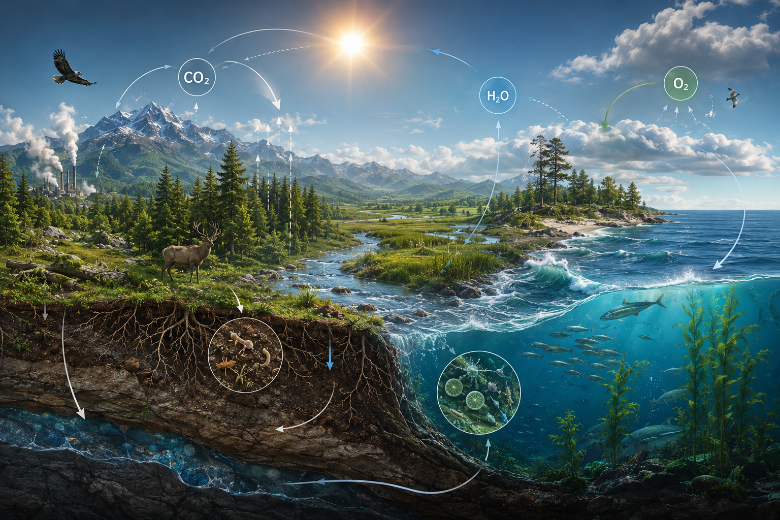
Biogeochemical cycles and the conditions of habitability examine how water, carbon, nitrogen, phosphorus, sulfur, oxygen, rock weathering, ocean chemistry, soils, sediments, and living metabolism interact to make Earth persistently livable. Habitability is not a static background condition. It is an achievement of coupled planetary processes that regulate climate, circulate nutrients, support primary production, maintain liquid water, buffer chemical extremes, sustain oxygen availability, and connect life to atmosphere, lithosphere, hydrosphere, cryosphere, and biosphere. Earth remains habitable not because its chemistry is fixed, but because matter continues to move through dynamic cycles that are buffered, transformed, delayed, stored, and renewed across time.
Biogeochemical cycles are central to biology because living systems do not merely occupy a chemically favorable planet. They participate in making and maintaining one. Photosynthesis draws carbon into biomass and releases oxygen. Respiration and decomposition return carbon to air, water, and soil. Microbes fix nitrogen, nitrify, denitrify, reduce sulfate, oxidize sulfur, mobilize phosphorus, and transform organic matter. Roots and fungi accelerate weathering and nutrient acquisition. Oceans absorb carbon, redistribute heat, and host vast photosynthetic communities. Sediments store carbon, phosphorus, sulfur, and other materials across long timescales. Through these processes, biology becomes geochemistry, and geochemistry becomes one of the foundations of life.
Main Library
Publications
Article Map
Biology
Related Topic
Environmental Science
Related Topic
Earth Science
Related Topic
Chemistry
The article is written for ecologists, marine biologists, freshwater scientists, medical and environmental-health readers, computational biology readers, biodiversity experts, microbiologists, soil scientists, Earth-system scientists, and research biologists who need a chemically grounded account of how life and Earth co-produce the conditions of persistence.
The article also extends biogeochemical science into quantitative and computational biology through mass-balance equations, multi-reservoir carbon and nutrient simulations, dissolved-oxygen stress models, habitability-support indicators, Monte Carlo uncertainty, scenario screening, R workflows, Python workflows, SQL provenance structures, and a linked full-stack GitHub repository containing Python, R, Julia, Fortran, Rust, Go, C, C++, SQL, notebooks, data files, and reproducibility documentation.
What biogeochemical cycles are
Biogeochemical cycles are the recurring movements and transformations of key elements and compounds through living organisms, air, water, soils, rocks, sediments, and oceans. They are “bio” because life mediates many of their transformations, “geo” because minerals, weathering, burial, sediments, and tectonic processes shape their long-term pathways, and “chemical” because the form an element takes determines how reactive, mobile, bioavailable, toxic, stable, or climatically influential it becomes.
The carbon cycle, water cycle, nitrogen cycle, phosphorus cycle, sulfur cycle, and oxygen cycle are among the most important because they help determine whether ecosystems can remain productive, whether climates remain temperate enough for liquid water, whether nutrients remain available to living systems, whether aquatic environments remain oxygenated, and whether complex aerobic life can persist. These cycles connect metabolism to planetary chemistry. They link root systems to weathering, microbes to nitrogen availability, plankton to oxygen production, soils to carbon storage, wetlands to methane and nutrient transformation, and oceans to climate regulation.
A scientifically serious treatment of these cycles has to resist two simplifications. The first is to imagine them as closed loops of elementary-school arrows. The second is to reduce them to purely geochemical processes that happen “in the environment” apart from biology. In reality, biogeochemical cycles are distributed networks of reservoirs, transformations, residence times, bottlenecks, feedbacks, delays, and thresholds. Their dynamics depend on microbial metabolism, ecosystem structure, hydrology, sedimentation, atmospheric transport, ocean circulation, soil development, rock weathering, and deep-time geological buffering all at once.
That is why biogeochemistry is not peripheral to biology. It is one of the deepest ways biology becomes planetary.
Why habitability is a cycling problem
A planet is not habitable simply because it contains water or the right temperature at a single moment. Habitability depends on whether key substances continue to circulate through stable but dynamic pathways. Water must move among ocean, atmosphere, ice, surface flow, soils, aquifers, and living systems. Carbon must cycle among life, air, ocean, soils, sediments, and rocks in ways that do not drive runaway heating or chemical collapse. Nutrients must be replenished, redistributed, transformed, retained, and released in forms that organisms can use. Oxygen must be produced, consumed, dissolved, circulated, and maintained at concentrations compatible with complex metabolism.
The condition of habitability is therefore inseparable from throughput, renewal, and buffering. Earth stays livable not because nothing changes, but because change remains organized within coupled cycles. The carbon cycle does not freeze atmospheric carbon dioxide at one perfect value; it regulates carbon through biological uptake, respiration, ocean exchange, sedimentation, weathering, and geological feedback. The water cycle does not hold freshwater in one permanent place; it redistributes water across atmosphere, land, ice, soils, rivers, aquifers, and oceans. The nitrogen cycle does not make nitrogen simply “available”; it transforms nitrogen among forms that differ profoundly in biological usefulness and environmental risk.
This point matters for research biologists as much as for Earth-system scientists. Organisms do not merely occupy chemically favorable conditions; they inherit and help reproduce those conditions. Photosynthesis, nitrogen fixation, decomposition, root-fungal interactions, plankton turnover, sediment burial, and weathering feedbacks all participate in the continual reconstruction of a habitable world. Habitability is therefore a systems outcome, not a static given.
Once framed this way, environmental disruption becomes easier to understand. A cycle driven too far from its historical range is not just an environmental anomaly. It is a destabilization of the chemical conditions under which living systems remain viable.
The water cycle and the mobility of life
The water cycle is the most immediate expression of planetary circulation. Water evaporates, condenses, falls as precipitation, infiltrates soils, recharges groundwater, flows through rivers and aquifers, freezes, melts, is taken up by organisms, transpired by plants, stored in snow and ice, and returned again to atmosphere and ocean. Habitability depends on this mobility because life requires not merely the presence of water, but the continuous delivery, storage, purification, and redistribution of water across landscapes, seasons, and ecological systems.
Water cycling also links climate, biology, and geology. It governs plant productivity, freshwater availability, soil moisture, erosion, sediment transport, aquifer recharge, wetland hydroperiod, and the transport of dissolved nutrients and pollutants. It connects forests to rainfall patterns, glaciers to river systems, wetlands to flood regulation, groundwater to long-term ecological persistence, and watersheds to estuaries and coastal seas. Hydrology is therefore not a neutral physical background. It is one of the operating conditions through which ecosystems remain alive.
Human activity now alters the water cycle through groundwater extraction, damming, land conversion, drainage, deforestation, irrigation, urbanization, contamination, and climate-driven changes in precipitation and snowpack. These disruptions can shift not only water availability but also salinity, sediment transport, nutrient delivery, dissolved oxygen, disease ecology, and thermal habitat. When hydrological cycling is disrupted, the consequences propagate through ecosystems rather than remaining confined to hydrology alone.
For ecologists and freshwater scientists, this means hydrology cannot be treated as background context. It is one of the causal architectures through which ecological structure is sustained or lost.
The carbon cycle and climate regulation
The carbon cycle is central to habitability because carbon is both a biological building block and a climate-regulating element. Carbon moves through fast pathways involving photosynthesis, respiration, decomposition, fire, food webs, and ocean-atmosphere exchange, and through slow pathways involving rock weathering, carbonate formation, sedimentation, burial, and tectonic cycling over millions of years. The balance between these pathways helps determine atmospheric carbon dioxide levels and therefore long-term climate conditions.
This makes the carbon cycle one of the clearest examples of biology and geology acting together. Plants and phytoplankton draw carbon into living tissue. Soils and sediments store or release it. Oceans absorb and redistribute it. Microbes decompose organic matter and return carbon to circulation. Rocks and weathering buffer carbon over geological time. Because some carbon compounds are greenhouse gases, disruption of the carbon cycle can quickly become disruption of climate itself.
Carbon is also central to ecosystem metabolism. Net primary production, respiration, decomposition, trophic transfer, soil organic matter formation, marine carbon export, and sediment burial all determine where carbon goes and how long it remains there. A forest, wetland, peatland, grassland, coral reef, agricultural soil, or coastal marsh is therefore not only a habitat. It is a carbon-processing system embedded in wider planetary flows.
For research biologists, the carbon cycle is not simply a global climate topic. It is a framework linking physiology, productivity, trophic structure, decomposition, ecosystem metabolism, biogeochemical storage, and climate regulation. Carbon is simultaneously molecular substrate, ecological currency, and climatic driver.
The nitrogen cycle and the problem of reactive fertility
Nitrogen is abundant in the atmosphere, but most organisms cannot use atmospheric nitrogen gas directly. The nitrogen cycle therefore depends on transformation. Nitrogen fixation converts inert atmospheric nitrogen into biologically available forms. Nitrification, assimilation, ammonification, denitrification, and anaerobic ammonium oxidation then move nitrogen through soils, waters, organisms, sediments, and back into the atmosphere. This cycle is one of the main reasons Earth can sustain high levels of productivity: life depends on reactive nitrogen, but habitability depends on keeping reactive nitrogen within ecologically workable bounds.
Modern disruption of the nitrogen cycle illustrates how habitability can be undermined by excess as well as scarcity. Reactive nitrogen supports fertility, but in excess it drives eutrophication, degraded habitat conditions, toxic blooms, altered species composition, nitrous oxide emissions, nitrate contamination, and low dissolved oxygen in freshwater, coastal, and estuarine systems. Synthetic fertilizer, fossil fuel combustion, manure management, wastewater, and agricultural intensification have greatly increased the amount of reactive nitrogen moving through land and water, making the nitrogen cycle a major site of human-driven Earth-system change.
Microbial ecology is essential here. The nitrogen cycle is not simply a chemical pathway. It is a microbial infrastructure. Bacteria and archaea mediate many of the transformations that determine whether nitrogen is fixed, retained, oxidized, reduced, lost as gas, or exported to downstream waters. Soil moisture, oxygen availability, organic matter, pH, temperature, plant uptake, and hydrological flow all influence which pathways dominate.
For microbiologists and soil biologists especially, nitrogen is one of the clearest examples of how microbial metabolism mediates planetary-scale consequences.
The phosphorus cycle and the constraint of rock-derived nutrients
Phosphorus differs from nitrogen in one decisive way: it has no large gaseous atmospheric reservoir analogous to atmospheric nitrogen. Much of its long-term cycling depends on rock weathering, soil processes, biological uptake, runoff, sediment transport, mineral sorption, erosion, and burial. This makes phosphorus simultaneously essential and often limiting. Primary production, ATP-based metabolism, nucleic acids, membranes, bone formation, and growth all depend on phosphorus, yet phosphorus availability is often tightly constrained by geological release rates, soil retention, hydrological transport, and biological demand.
Because phosphorus is so tightly linked to weathering and erosion, it provides a particularly vivid example of how geology and biology constrain one another. A planet can have sunlight, water, and carbon, yet still be biologically constrained if nutrient release and redistribution are too limited or poorly timed. Phosphorus limitation can structure ecosystems, affect plant productivity, influence microbial metabolism, and constrain carbon uptake in some regions.
At the same time, oversupply of phosphorus to aquatic systems can destabilize ecological structure, especially when nutrient loading exceeds the assimilative and buffering capacity of receiving waters. Phosphorus enrichment can fuel algal blooms, cyanobacterial dominance, oxygen depletion, altered food webs, and water-quality impairment. Like nitrogen, phosphorus is therefore a nutrient whose ecological effect depends on context, form, timing, pathway, and concentration.
For plant biologists, microbial ecologists, freshwater scientists, and Earth-system modelers, phosphorus remains one of the most important reminder variables: productivity is never just a matter of carbon alone.
The sulfur cycle, redox chemistry, and environmental transformation
The sulfur cycle is less publicly discussed than water or carbon, but it is fundamental to redox chemistry, mineral formation, microbial metabolism, sedimentary processes, atmospheric chemistry, and Earth’s deep-time environmental history. Sulfur moves among rocks, volcanic emissions, marine sulfate, soils, organisms, wetlands, sediments, hydrothermal systems, aerosols, and microbial pathways such as sulfate reduction and sulfide oxidation. These transformations affect acidity, metal mobility, sediment chemistry, atmospheric particles, and the energy economies of microbial ecosystems.
Sulfur also matters because it links deep-time Earth history to present-day environmental conditions. Variations in sulfur speciation and isotopes can record redox environments, biological activity, hydrothermal influence, and changes in ocean-atmosphere chemistry. In modern systems, sulfur cycling helps determine whether sediments remain oxic or anoxic, whether toxic sulfide accumulates, how wetlands and estuaries process organic matter, and how microbial life reorganizes matter in low-oxygen environments.
Redox gradients are especially important. In oxygen-rich settings, sulfur tends to occupy different chemical pathways than it does in anoxic sediments, wetlands, or deep marine environments. Microbes use these gradients as energy landscapes, and their metabolism can determine whether sulfur compounds are oxidized, reduced, immobilized, released, or coupled to other cycles such as carbon, iron, and nitrogen.
For marine biologists and microbial ecologists, sulfur cycling is especially important in transitional and low-oxygen systems where redox gradients drive both ecological constraint and biogeochemical novelty.
The oxygen cycle and the chemistry of complex life
The oxygen cycle matters because oxygen is both a product of photosynthetic life and a precondition for most complex aerobic metabolism. Photosynthetic organisms release oxygen, while respiration, decomposition, oxidation, combustion, and chemical weathering consume it. Earth’s atmospheric oxygen is therefore not simply “there.” It is maintained through long-term balances among biological production, organic carbon burial, reduced mineral oxidation, respiration, and geological processes.
Oxygen is equally important in water. Dissolved oxygen helps determine aquatic habitability for fish, invertebrates, microbes, and whole food webs. Low-oxygen conditions have major biogeochemical consequences and can worsen under some combinations of nutrient loading, stratification, warming, and organic matter decomposition. Oxygen cycling therefore links metabolism, stratification, eutrophication, warming, and habitat viability.
The oxygen cycle also clarifies why habitability is spatially variable. Oxygen may be abundant in the atmosphere while scarce in bottom waters, sediments, wetlands, hypoxic estuaries, stratified lakes, or oxygen minimum zones. To think about habitability seriously is to ask not only whether oxygen exists, but where, in what form, at what concentration, and under what ecological stresses.
For medical and environmental-health readers, oxygen decline also has downstream implications for water quality, toxins, fish kills, harmful blooms, contamination dynamics, and exposure environments.
Weathering, soils, and long-term planetary buffering
Rock weathering and soil formation are among the quiet foundations of habitability. Weathering releases mineral nutrients, shapes alkalinity, affects river chemistry, contributes to long-term carbon regulation, and helps move carbon from atmosphere into bicarbonate, carbonate minerals, and sediments. Soils, meanwhile, are not inert containers. They are reactive interfaces where minerals, roots, fungi, microbes, organic matter, water, and gases meet. Many of the most important transformations in nitrogen, phosphorus, sulfur, and carbon cycling occur in soils or at soil-water boundaries.
This is one reason habitability is best understood as a coupled Earth-surface process. The conditions that allow plant growth, microbial decomposition, nutrient retention, groundwater recharge, atmospheric exchange, and ecosystem recovery all depend on the long interaction of climate, rock, relief, biology, and time. Weathering is not merely geological erosion. It is part of the chemical infrastructure through which nutrient availability, alkalinity, and long-term carbon buffering emerge.
Soils are especially important because they integrate biological and geochemical processes in a zone of intense transformation. They store carbon, retain nutrients, support root systems, host microbial communities, regulate water, and mediate gas exchange. When soils erode, compact, acidify, salinize, contaminate, or lose organic matter, the damage is not merely agricultural. It is biogeochemical. The cycle interfaces that sustain fertility and buffering begin to fail.
For research biologists, soils should not be treated as support medium alone. They are active chemical and biological processors within the planetary life-support system.
Oceans, sediments, and the long memory of the Earth system
The ocean is one of the largest active reservoirs in multiple global cycles. It stores and redistributes heat, absorbs carbon dioxide, produces much of Earth’s oxygen through marine photosynthesis, and mediates nutrient transformations across surface waters, deep waters, coastlines, continental shelves, and sediments. Ocean uptake of carbon is essential to the global carbon cycle but chemically consequential, because dissolved carbon dioxide changes seawater chemistry and lowers pH over time.
Marine biogeochemistry is also structured by vertical and horizontal movement. Nutrients are consumed in sunlit surface waters, exported downward in organic matter, remineralized at depth, and returned to the surface through mixing and upwelling. Oxygen is produced near the surface but consumed throughout the water column and sediments. Carbon is exchanged with the atmosphere, incorporated into organisms, dissolved in seawater, exported through the biological pump, and stored in deep waters or sediments. These pathways determine the ocean’s role in climate regulation, fisheries, oxygen stability, and habitat quality.
Sediments give the Earth system memory. Burial can sequester carbon, phosphorus, sulfur, and other materials over long timescales. Sediment release can also return nutrients or reduced compounds to active circulation under changing oxygen or redox conditions. In this sense, habitability is not just the property of active surface fluxes. It also depends on reservoirs, lags, buffering capacities, and the delayed consequences of past deposition, erosion, burial, and chemical transformation.
This long memory is one of the reasons Earth-system behavior often includes thresholds, hysteresis, and delayed response rather than immediate equilibrium adjustment.
Biology as a geochemical force
Life does not merely receive the products of these cycles. It actively shapes them. Plants alter water fluxes through transpiration and control large portions of land carbon uptake. Microbes fix nitrogen, nitrify, denitrify, reduce sulfate, oxidize sulfur, decompose organic matter, mobilize phosphorus, and help regulate methane. Phytoplankton affect carbon sequestration, oxygen production, marine food webs, and ocean chemistry. Fungi and roots accelerate mineral weathering and nutrient acquisition. Earth’s habitability is therefore co-produced by organisms acting as planetary chemical agents.
This is why biogeochemical cycles belong just as much to biology as to geochemistry. The biosphere is not separate from the Earth system; it is one of its active engines. The structure of ecosystems, the traits of organisms, and the metabolic capacities of microbes all influence how elements move, where they accumulate, and what forms of habitability are maintained or lost.
The phrase “biology as a geochemical force” is not metaphorical. It describes literal planetary work. Cyanobacteria and photosynthesis transformed Earth’s oxygen history. Plants changed weathering, soils, carbon storage, and hydrology. Microbes created and maintained major metabolic pathways in nitrogen, sulfur, methane, iron, and carbon cycling. Plankton help regulate marine carbon flow and oxygen production. Fungi, roots, and soil organisms shape mineral weathering and nutrient turnover.
For research biologists, that means biogeochemistry is not a neighboring discipline. It is one of the scales at which biology reveals its full planetary consequence.
Disruption, eutrophication, acidification, and biogeochemical overshoot
Human activity now alters nearly every major biogeochemical cycle. Fossil fuel combustion reshapes the carbon cycle and climate. Fertilizer use and industrial nitrogen fixation intensify reactive nitrogen flows. Agricultural runoff and wastewater increase phosphorus delivery to freshwaters and coasts. Carbon dioxide uptake changes ocean acidity. Land-use change, damming, groundwater depletion, deforestation, wetland drainage, soil degradation, and urbanization alter the water cycle. These are not isolated environmental problems. They are disruptions in the fundamental circulations that maintain habitability.
Eutrophication and acidification show how quickly these disruptions can cascade. Excess nutrient loading can trigger algal blooms, oxygen depletion, habitat degradation, fish kills, toxin production, altered species composition, and food-web change. Excess carbon dioxide can alter ocean carbonate chemistry and threaten calcifying organisms. Reduced oxygen can transform sediment chemistry and release nutrients or toxic compounds. The logic is the same in each case: when key cycles are driven too far from their historically regulating ranges, the environments they sustain become less stable, less buffered, and less supportive of complex life.
Biogeochemical overshoot is especially dangerous because cycle disruptions interact. Nutrient loading can worsen oxygen depletion. Warming can intensify stratification and reduce oxygen solubility. Land-use change can increase erosion, carbon release, and nutrient export. Ocean acidification can combine with warming and deoxygenation to stress marine organisms. Soil degradation can weaken carbon storage, water retention, and fertility simultaneously.
For marine scientists, ecologists, freshwater scientists, and environmental-health readers, this is where biogeochemistry becomes unmistakably practical. Chemistry becomes habitat fate.
Planetary boundaries and the limits of stable cycling
The planetary boundaries framework is especially important here because it treats Earth’s stability as dependent on a limited number of critical processes, including climate change, freshwater change, ocean acidification, and biogeochemical flows. In recent updates, scientists have concluded that several boundaries have been transgressed, including biogeochemical flows. This does not mean that Earth suddenly becomes uninhabitable. It means that core regulating processes have been pushed outside the conditions associated with the relatively stable Earth-system state in which complex societies and many ecosystems developed.
This framework matters because it makes habitability legible as a question of regulated limits rather than generic environmental concern. The issue is not simply that humans affect cycles. All organisms affect cycles. The issue is whether those effects push core regulating processes beyond ranges compatible with resilience, ecological function, and long-term stability. Biogeochemical cycles are therefore not background chemistry. They are part of the planetary operating system of habitability.
The framework also makes clear that boundaries interact. Biogeochemical flows influence freshwater quality, coastal oxygen, ocean chemistry, land systems, biodiversity, and climate feedbacks. Climate change influences water cycling, oxygen demand, soil carbon, weathering, nutrient availability, and ecosystem metabolism. Biosphere integrity affects carbon uptake, nutrient retention, hydrology, and resilience. These interactions are why isolated environmental management often fails. Cycles must be understood as coupled systems.
For scientists, one of the framework’s most useful features is that it encourages systems-level reasoning about interaction among boundaries rather than isolated topic silos.
Quantitative Earth-system thinking: mathematics, R, and Python
Biogeochemical cycles are especially well suited to quantitative treatment because they are fundamentally about stocks, flows, reservoirs, transformations, and feedbacks. A simple carbon balance can be expressed as:
\Delta C=\text{inputs}-\text{outputs}
\]
Interpretation: This compact balance expresses the stock-flow logic behind carbon accounting. It is useful as a conceptual scaffold, but real Earth-system balances require linked compartments, uncertain fluxes, chemical forms, residence times, and feedbacks.
Real Earth-system balances require many linked compartments:
\frac{dC_{atm}}{dt}=E_{fossil}+E_{land}+E_{dist}-U_{land}-U_{ocean}
\]
Interpretation: Atmospheric carbon changes as fossil emissions, land-use emissions, and disturbance releases are offset or amplified by land and ocean uptake. The expression makes clear that atmospheric carbon burden depends not only on emissions, but also on the capacity of land and ocean systems to absorb, transform, or later re-release carbon.
A more general research-facing mass-balance form for any reservoir \(X\) can be written as:
\frac{dX}{dt}=\sum I_j-\sum O_k+\sum T_m
\]
Interpretation: \(I_j\) represents external inputs, \(O_k\) represents external outputs, and \(T_m\) represents internal transformations that change the form, location, bioavailability, or climatic relevance of the substance. This is useful because the same element can move through multiple compartments while changing state.
For nutrient-loaded aquatic systems, a compact oxygen-demand formulation might also be written as:
\frac{dO}{dt}=P_O-R_O-D_O-S_O
\]
Interpretation: \(O\) is dissolved oxygen, \(P_O\) is oxygen production, \(R_O\) is respiration demand, \(D_O\) is decomposition-driven oxygen demand, and \(S_O\) is stratification or exchange limitation. This is not a full lake or estuary model, but it captures a central idea: oxygen conditions are emergent properties of multiple coupled processes rather than one direct driver.
Worked example: carbon balance
Suppose fossil emissions are \(E_{fossil}=10.0\), land-use emissions are \(E_{land}=1.0\), disturbance emissions are \(E_{dist}=0.5\), land uptake is \(U_{land}=3.0\), and ocean uptake is \(U_{ocean}=2.6\), all expressed in a simplified common carbon unit. Then:
\frac{dC_{atm}}{dt}=10.0+1.0+0.5-3.0-2.6=5.9
\]
Interpretation: The simplified result means that 5.9 units remain as a net atmospheric increment. The value is not a full carbon-cycle model, but it shows why biosphere and ocean uptake matter: changes in land uptake, ocean uptake, disturbance release, or emissions can alter atmospheric carbon outcomes.
These equations do not replace empirical biogeochemistry, field chemistry, ocean observation, microbial process measurements, or Earth-system models. They clarify the stock-flow and transformation logic that underlies serious biogeochemical analysis.
R and Python workflows
The following examples are compact article-level workflows. The full GitHub repository expands them into richer multi-language implementations with SQL provenance, validation notes, multi-reservoir simulations, dissolved-oxygen stress models, nutrient-loading scenarios, habitability-risk screening, uncertainty envelopes, and reproducible computational biogeochemistry scaffolding.
R example: multi-reservoir carbon and nutrient flux simulation
# Multi-reservoir biogeochemical simulation
#
# This prototype tracks carbon and reactive nitrogen across atmosphere, land,
# ocean, and a coastal receiving system under uncertain uptake and nutrient
# loading. It is compact enough for an article but structured enough to extend.

set.seed(42)

simulate_biogeochem <- function(
  years = 60,
  n_sims = 500,
  fossil_start = 10,
  fossil_growth = 0.008,
  land_uptake_mean = 3.0,
  land_uptake_sd = 0.4,
  ocean_uptake_mean = 2.6,
  ocean_uptake_sd = 0.3,
  disturbance_mean = 0.5,
  disturbance_sd = 0.2,
  reactive_n_start = 1.0,
  reactive_n_growth = 0.015,
  coastal_assimilation_mean = 0.65,
  coastal_assimilation_sd = 0.08
) {
  atm_carbon <- matrix(NA_real_, nrow = years, ncol = n_sims)
  coastal_n_surplus <- matrix(NA_real_, nrow = years, ncol = n_sims)

  for (sim in seq_len(n_sims)) {
    carbon_state <- 0
    nitrogen_state <- 0

    for (year in seq_len(years)) {
      fossil_t <- fossil_start * (1 + fossil_growth)^(year - 1)
      land_uptake_t <- max(0, rnorm(1, land_uptake_mean, land_uptake_sd))
      ocean_uptake_t <- max(0, rnorm(1, ocean_uptake_mean, ocean_uptake_sd))
      disturbance_t <- max(0, rnorm(1, disturbance_mean, disturbance_sd))

      reactive_n_t <- reactive_n_start * (1 + reactive_n_growth)^(year - 1)
      coastal_assimilation_t <- min(
        1,
        max(0, rnorm(1, coastal_assimilation_mean, coastal_assimilation_sd))
      )

      # Carbon increment to atmosphere.
      carbon_increment <- fossil_t + disturbance_t -
        land_uptake_t - ocean_uptake_t

      carbon_state <- carbon_state + carbon_increment

      # Reactive nitrogen surplus reaching coastal system.
      n_surplus <- reactive_n_t * (1 - coastal_assimilation_t)
      nitrogen_state <- nitrogen_state + n_surplus

      atm_carbon[year, sim] <- carbon_state
      coastal_n_surplus[year, sim] <- nitrogen_state
    }
  }

  list(
    atm_carbon = atm_carbon,
    coastal_n_surplus = coastal_n_surplus,
    carbon_mean = rowMeans(atm_carbon),
    carbon_q05 = apply(atm_carbon, 1, quantile, probs = 0.05),
    carbon_q95 = apply(atm_carbon, 1, quantile, probs = 0.95),
    nitrogen_mean = rowMeans(coastal_n_surplus),
    nitrogen_q05 = apply(coastal_n_surplus, 1, quantile, probs = 0.05),
    nitrogen_q95 = apply(coastal_n_surplus, 1, quantile, probs = 0.95)
  )
}

res <- simulate_biogeochem()

years <- seq_len(nrow(res$atm_carbon))

plot(
  years,
  res$carbon_mean,
  type = "l",
  lwd = 2,
  xlab = "Year",
  ylab = "Cumulative atmospheric carbon burden",
  main = "Carbon Burden Scenario"
)

lines(years, res$carbon_q05, lty = 2)
lines(years, res$carbon_q95, lty = 2)

cat("Final year mean carbon burden:", round(tail(res$carbon_mean, 1), 3), "\n")
cat("Final year mean nitrogen surplus:", round(tail(res$nitrogen_mean, 1), 3), "\n")
This R workflow is more useful than a static balance equation because it introduces multiple reservoirs, cumulative effects, uncertainty envelopes, and linked carbon-nutrient dynamics. A research biologist or Earth-system scientist could adapt it for watershed export, estuarine loading, forest disturbance, restoration scenarios, soil carbon recovery, or climate-nutrient interaction studies.
Python example: coupled habitability-risk screening framework
import numpy as np
import pandas as pd

# Example ecological or regional units.
# Each indicator is normalized from 0 to 1 for demonstration.
units = pd.DataFrame(
    {
        "unit": ["A", "B", "C", "D", "E"],
        "carbon_uptake_capacity": [0.82, 0.66, 0.51, 0.88, 0.59],
        "water_regulation": [0.79, 0.62, 0.48, 0.85, 0.55],
        "nitrogen_retention": [0.75, 0.58, 0.36, 0.81, 0.49],
        "phosphorus_buffering": [0.73, 0.61, 0.42, 0.79, 0.46],
        "oxygen_stability": [0.84, 0.67, 0.39, 0.87, 0.53],
        "disturbance_pressure": [0.24, 0.40, 0.74, 0.18, 0.58],
        "acidification_pressure": [0.21, 0.35, 0.69, 0.14, 0.51],
        "nutrient_loading": [0.28, 0.46, 0.81, 0.20, 0.63],
    }
)

# Composite habitability-support score.
# Positive variables represent buffering or support capacity.
# Negative variables represent pressures that weaken habitability.
units["habitability_support"] = (
    0.18 * units["carbon_uptake_capacity"]
    + 0.16 * units["water_regulation"]
    + 0.14 * units["nitrogen_retention"]
    + 0.14 * units["phosphorus_buffering"]
    + 0.16 * units["oxygen_stability"]
    - 0.10 * units["disturbance_pressure"]
    - 0.06 * units["acidification_pressure"]
    - 0.06 * units["nutrient_loading"]
)

# Risk classification.
conditions = [
    units["habitability_support"] >= 0.65,
    (units["habitability_support"] >= 0.45)
    & (units["habitability_support"] < 0.65),
    units["habitability_support"] < 0.45,
]

labels = ["relatively-buffered", "stressed", "high-risk"]

units["risk_class"] = np.select(conditions, labels, default="unknown")

# Scenario: intensified nutrient loading and warming-linked oxygen stress.
units["oxygen_stability_scenario"] = units["oxygen_stability"] - 0.10
units["nutrient_loading_scenario"] = units["nutrient_loading"] + 0.12

units["habitability_support_scenario"] = (
    0.18 * units["carbon_uptake_capacity"]
    + 0.16 * units["water_regulation"]
    + 0.14 * units["nitrogen_retention"]
    + 0.14 * units["phosphorus_buffering"]
    + 0.16 * units["oxygen_stability_scenario"]
    - 0.10 * units["disturbance_pressure"]
    - 0.06 * units["acidification_pressure"]
    - 0.06 * units["nutrient_loading_scenario"]
)

units["delta_scenario"] = (
    units["habitability_support_scenario"]
    - units["habitability_support"]
)

print(
    units[
        [
            "unit",
            "habitability_support",
            "risk_class",
            "habitability_support_scenario",
            "delta_scenario",
        ]
    ].round(3).to_string(index=False)
)
This Python workflow is useful because it treats habitability-support capacity as a composite systems variable, introduces multiple coupled pressures, and includes a scenario stress test. It can be extended with field chemistry, remote-sensing indicators, eDNA signals, dissolved oxygen data, watershed nutrient budgets, marine carbonate chemistry, soil carbon metrics, microbial process proxies, and water-quality monitoring networks. For research biologists and computational readers, that makes it closer to a real screening and prioritization framework than a classroom illustration.
Python example: dissolved-oxygen stress screening
import numpy as np
import pandas as pd

# Demonstration dataset for aquatic systems.
# Values are simplified and normalized for article readability.
waterbodies = pd.DataFrame(
    {
        "site": ["lake_A", "estuary_B", "river_C", "lagoon_D", "wetland_E"],
        "oxygen_production": [0.72, 0.60, 0.66, 0.48, 0.58],
        "respiration_demand": [0.34, 0.49, 0.38, 0.62, 0.51],
        "decomposition_demand": [0.28, 0.55, 0.31, 0.70, 0.48],
        "stratification_limitation": [0.20, 0.52, 0.18, 0.65, 0.42],
        "nutrient_loading": [0.31, 0.68, 0.40, 0.81, 0.57],
    }
)

waterbodies["oxygen_stability_index"] = (
    0.45 * waterbodies["oxygen_production"]
    - 0.20 * waterbodies["respiration_demand"]
    - 0.18 * waterbodies["decomposition_demand"]
    - 0.12 * waterbodies["stratification_limitation"]
    - 0.05 * waterbodies["nutrient_loading"]
)

waterbodies["oxygen_stress_class"] = pd.cut(
    waterbodies["oxygen_stability_index"],
    bins=[-1, 0.05, 0.20, 1],
    labels=["high-stress", "moderate-stress", "lower-stress"],
)

# Scenario: warming and nutrient enrichment.
waterbodies["oxygen_stability_warming_scenario"] = (
    0.45 * (waterbodies["oxygen_production"] - 0.05)
    - 0.20 * (waterbodies["respiration_demand"] + 0.08)
    - 0.18 * (waterbodies["decomposition_demand"] + 0.08)
    - 0.12 * (waterbodies["stratification_limitation"] + 0.10)
    - 0.05 * (waterbodies["nutrient_loading"] + 0.10)
)

waterbodies["delta_under_scenario"] = (
    waterbodies["oxygen_stability_warming_scenario"]
    - waterbodies["oxygen_stability_index"]
)

print(
    waterbodies[
        [
            "site",
            "oxygen_stability_index",
            "oxygen_stress_class",
            "oxygen_stability_warming_scenario",
            "delta_under_scenario",
        ]
    ].round(3).to_string(index=False)
)
This dissolved-oxygen scaffold makes eutrophication, warming, decomposition, and stratification visible as coupled pressures rather than isolated variables. A full workflow could connect this structure to sensor data, lake profiles, estuarine monitoring, marine oxygen observations, nutrient records, or restoration scenarios.
These examples are still compact enough to fit inside an article, but they move toward the kinds of workflows scientists actually use: mass-balance reasoning, multi-reservoir modeling, uncertainty, composite system indicators, explicit scenario testing, dissolved-oxygen stress screening, and reproducible computational structure.
GitHub repository
The article body includes compact R and Python examples so the ecological and scientific argument remains readable. The full repository expands those examples into a broader computational biogeochemistry workflow, including multi-reservoir carbon and nutrient simulations, habitability-risk screening, dissolved-oxygen stress modeling, nutrient-loading scenarios, SQL provenance structures, reproducible data files, and full-stack scientific-computing examples across Python, R, Julia, Fortran, Rust, Go, C, C++, SQL, and notebooks.
Why this matters for scientific work
Biogeochemical cycles and the conditions of habitability matter across ecology, climate science, microbiology, soil biology, marine biology, freshwater biology, restoration ecology, agroecology, conservation biology, physiology, environmental health, and Earth-system governance because all of these fields depend on how matter moves through life and environment. For ecologists, the article clarifies that productivity, resilience, and biodiversity are inseparable from chemical throughput. For marine biologists, it makes clear that ocean carbon uptake, oxygen stability, coastal nutrient loading, carbonate chemistry, and sediment processes are central rather than secondary to marine life. For freshwater scientists, it shows why rivers, lakes, wetlands, floodplains, and aquifers are chemical as well as ecological systems.
For medical and environmental-health readers, biogeochemistry shows how water quality, harmful blooms, oxygen decline, contamination, nitrate exposure, acidification, and hypoxia are environmental conditions before they become public-health realities. For computational and biotechnology-oriented readers, it demonstrates why modern biogeochemistry increasingly depends on linked datasets, models, sensors, reproducible workflows, and systems-level indicators. For research biologists more broadly, it situates organismal metabolism, microbial transformation, ecosystem process, and Earth-system chemistry inside one shared scientific framework.
This makes biogeochemical literacy indispensable to any serious account of living systems. It clarifies that habitability is neither automatic nor permanent. It is reproduced through circulation, transformation, renewal, feedback, and constraint. When those processes are destabilized, the damage appears in crops, reefs, rivers, forests, fisheries, soils, disease dynamics, coastal waters, and climate itself.
Conclusion
Biogeochemical cycles are among the deepest foundations of habitability because they connect life to the larger Earth system through recurring pathways of water, carbon, nutrients, gases, minerals, redox chemistry, and biologically mediated transformation. They make fertility possible, regulate climate, support metabolism, structure ecosystems, maintain oxygen availability, and buffer planetary conditions over timescales ranging from seconds to millions of years. Earth remains livable not because it is chemically static, but because its major cycles continue to circulate matter through connected reservoirs in ways that sustain dynamic but bounded stability.
To understand biogeochemical cycles is therefore to understand one of the central truths of biology and Earth-system science alike: life persists only because the planet continues to move, transform, and renew the materials of life. Where that circulation remains organized, habitability persists. Where it is pushed beyond stable bounds, the conditions of living systems begin to fail.
Biogeochemistry makes visible the chemical architecture beneath ecology. It shows that a forest is carbon, water, nitrogen, phosphorus, oxygen, soil, fungi, microbes, and weathering as much as trunks and leaves. It shows that an estuary is hydrology, nutrients, sediments, oxygen, salinity, plankton, microbes, and tidal exchange as much as water and shoreline. It shows that habitability is not a possession of the planet but an ongoing planetary process.
Related articles
- Biology
- Ecology and the Interdependence of Life
- Population Dynamics and Ecological Modeling
- Populations, Communities, and Ecosystem Dynamics
- Biodiversity and the Structure of Living Systems
- The Biosphere and Planetary Life Support Systems
- Biomes, Habitats, and the Geography of Life
- Plant Biology and the Life of Primary Producers
- Microbiology and the Hidden Majority of Life
- Fungi and the Networks of Decomposition and Exchange
- Physiology and the Regulation of Living Systems
Further reading
- NASA Earth Observatory (2011) The Carbon Cycle. Available at: https://science.nasa.gov/earth/earth-observatory/the-carbon-cycle/
- NASA Terra (n.d.) Carbon Cycle and Ecosystems. Available at: https://terra.nasa.gov/science/carbon-cycle-and-ecosystems
- U.S. Geological Survey (n.d.) Learn About Water. Available at: https://www.usgs.gov/water-science-school/learn-about-water
- U.S. Geological Survey (2025) Interactive Water Cycle Diagram. Available at: https://water.usgs.gov/edu/watercycle-kids-adv.html
- NOAA Ocean Service (2024) What Is Ocean Acidification? Available at: https://oceanservice.noaa.gov/facts/acidification.html
- NOAA Ocean Service (2024) How Much Oxygen Comes from the Ocean? Available at: https://oceanservice.noaa.gov/facts/ocean-oxygen.html
- U.S. Environmental Protection Agency (n.d.) Basic Information on Nutrient Pollution. Available at: https://www.epa.gov/nutrientpollution/basic-information-nutrient-pollution
- Stockholm Resilience Centre (n.d.) Planetary Boundaries. Available at: https://www.stockholmresilience.org/research/planetary-boundaries.html
- Richardson, K. et al. (2023) ‘Earth beyond six of nine planetary boundaries’, Science Advances, 9(37), eadh2458. Available at: https://www.science.org/doi/10.1126/sciadv.adh2458
- Falkowski, P.G., Fenchel, T. and Delong, E.F. (2008) ‘The microbial engines that drive Earth’s biogeochemical cycles’, Science, 320(5879), pp. 1034–1039. Available at: https://doi.org/10.1126/science.1153213
References
- Falkowski, P.G., Fenchel, T. and Delong, E.F. (2008) ‘The microbial engines that drive Earth’s biogeochemical cycles’, Science, 320(5879), pp. 1034–1039. Available at: https://doi.org/10.1126/science.1153213
- Falkowski, P.G., Barber, R.T. and Smetacek, V. (1998) ‘Biogeochemical controls and feedbacks on ocean primary production’, Science, 281(5374), pp. 200–206. Available at: https://doi.org/10.1126/science.281.5374.200
- Field, C.B., Behrenfeld, M.J., Randerson, J.T. and Falkowski, P. (1998) ‘Primary production of the biosphere: Integrating terrestrial and oceanic components’, Science, 281(5374), pp. 237–240. Available at: https://doi.org/10.1126/science.281.5374.237
- NASA Earth Observatory (2011) The Carbon Cycle. Available at: https://science.nasa.gov/earth/earth-observatory/the-carbon-cycle/
- NASA Terra (n.d.) Carbon Cycle and Ecosystems. Available at: https://terra.nasa.gov/science/carbon-cycle-and-ecosystems
- NOAA (2022) Ocean Acidification. Available at: https://www.noaa.gov/ocean-acidification
- NOAA Global Ocean Monitoring and Observing (n.d.) Ocean Carbon and Biogeochemistry. Available at: https://globalocean.noaa.gov/the-ocean/ocean-carbon-biogeochemistry/
- NOAA Ocean Service (2024) What Is Ocean Acidification? Available at: https://oceanservice.noaa.gov/facts/acidification.html
- NOAA Ocean Service (2024) How Much Oxygen Comes from the Ocean? Available at: https://oceanservice.noaa.gov/facts/ocean-oxygen.html
- NOAA Geophysical Fluid Dynamics Laboratory (n.d.) Will Open Ocean Oxygen Stress Intensify under Climate Change? Available at: https://www.gfdl.noaa.gov/open-ocean-oxygen-stress-intensification/
- NOAA National Centers for Coastal Ocean Science (2018) Oxygen: Dynamics and Biogeochemical Consequences. Available at: https://coastalscience.noaa.gov/data_reports/oxygen-dynamics-and-biogeochemical-consequences/
- Richardson, K. et al. (2023) ‘Earth beyond six of nine planetary boundaries’, Science Advances, 9(37), eadh2458. Available at: https://www.science.org/doi/10.1126/sciadv.adh2458
- Rockström, J. et al. (2009) ‘A safe operating space for humanity’, Nature, 461, pp. 472–475. Available at: https://doi.org/10.1038/461472a
- Schlesinger, W.H. and Bernhardt, E.S. (2020) Biogeochemistry: An Analysis of Global Change. 4th edn. London: Academic Press. Publisher information available at: https://www.elsevier.com/books/biogeochemistry/schlesinger/978-0-12-814608-8
- Steffen, W. et al. (2015) ‘Planetary boundaries: Guiding human development on a changing planet’, Science, 347(6223), 1259855. Available at: https://doi.org/10.1126/science.1259855
- Stockholm Resilience Centre (n.d.) Planetary Boundaries. Available at: https://www.stockholmresilience.org/research/planetary-boundaries.html
- U.S. Environmental Protection Agency (n.d.) Basic Information on Nutrient Pollution. Available at: https://www.epa.gov/nutrientpollution/basic-information-nutrient-pollution
- U.S. Environmental Protection Agency (2025) Indicators: Nitrogen. Available at: https://www.epa.gov/national-aquatic-resource-surveys/indicators-nitrogen
- U.S. Geological Survey (n.d.) Learn About Water. Available at: https://www.usgs.gov/water-science-school/learn-about-water
- U.S. Geological Survey (2025) Interactive Water Cycle Diagram. Available at: https://water.usgs.gov/edu/watercycle-kids-adv.html
- U.S. Geological Survey (n.d.) Phosphorus and Water. Available at: https://www.usgs.gov/water-science-school/science/phosphorus-and-water
- U.S. Geological Survey (2024) Characterizing Sulfur Redox State and Geochemical Implications through Deep Time Using Mineral Records. Available at: https://www.usgs.gov/publications/characterizing-sulfur-redox-state-and-geochemical-implications-deep-time-using-mineral