Equilibrium and the Dynamics of Reversible Systems

Last Updated May 28, 2026

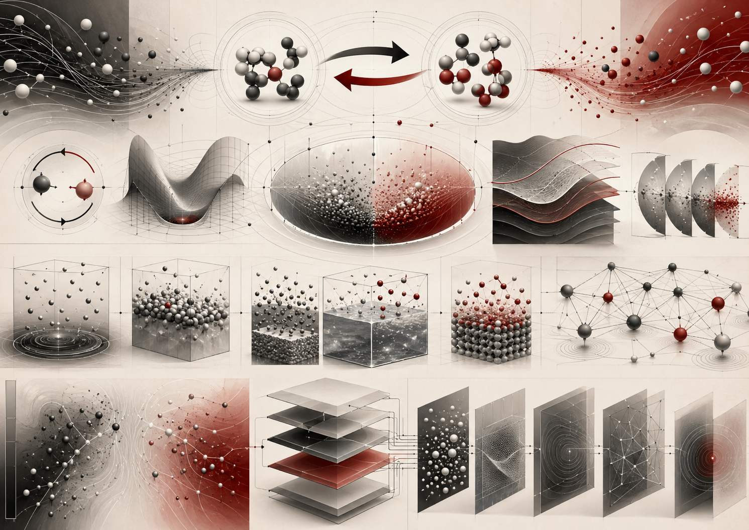
Chemical equilibrium is not stillness. It is dynamic balance. In a reversible chemical system, reactants form products while products simultaneously reform reactants. At equilibrium, the forward and reverse processes continue, but their rates balance so that macroscopic composition no longer changes. The system is active at the molecular scale while appearing stable at the observable scale.

The central thesis of this article is that equilibrium is a framework for understanding how chemical systems respond to constraint, perturbation, composition, temperature, pressure, phase, solvent, activity, and molecular interaction. Equilibrium describes both the tendency toward balance and the structured ways in which balance shifts when conditions change.

Equilibrium chemistry sits at the center of chemical reasoning because it connects thermodynamics, kinetics, concentration, activity, pressure, phase, solubility, acid-base behavior, complex formation, precipitation, gas reactions, biochemical regulation, environmental chemistry, and industrial process design. Stoichiometry tells how substances are related by balanced equations. Thermodynamics explains why equilibrium has a particular direction and composition. Kinetics explains how the system approaches that composition through time. Equilibrium brings these perspectives together.

Why Equilibrium Matters

Equilibrium matters because many chemical systems do not proceed completely from reactants to products. Instead, they settle into mixtures shaped by reversible reaction, thermodynamic driving force, temperature, pressure, concentration, phase, solvent, and molecular interaction. A reaction can be strongly product-favored, weakly product-favored, reactant-favored, pressure-sensitive, temperature-sensitive, pH-sensitive, activity-sensitive, or coupled to other equilibria.

This makes equilibrium central to chemistry. Acid-base systems depend on proton-transfer equilibria. Solubility depends on dissolution and precipitation equilibria. Complex formation depends on ligand binding equilibria. Gas reactions depend on partial pressures and equilibrium constants. Biochemistry depends on binding, folding, protonation, redox, and metabolic equilibria. Environmental chemistry depends on carbonate systems, metal speciation, partitioning, adsorption, gas exchange, and mineral equilibria. Industrial chemistry depends on shifting equilibria toward useful products while balancing energy, cost, selectivity, rate, and safety.

Equilibrium also shows why chemistry is conditional. A reaction mixture that is stable at one temperature may shift at another. A gas equilibrium may respond to pressure. A precipitate may dissolve if complexing ligands are added. A weak acid may change ionization behavior depending on pH. A biological binding interaction may depend on ligand concentration and competing equilibria.

Equilibrium reasoning is especially important because it prevents one-way thinking. A chemical equation may be written with a forward arrow for convenience, but many systems retain the possibility of reverse change. Products may decompose, ions may recombine, gases may redissolve, ligands may dissociate, proteins may unfold, minerals may precipitate again, and adsorbed molecules may desorb.

For researchers and scientists, chemical equilibrium is therefore not a static endpoint. It is a structured response of matter to conditions, constraints, perturbations, and thermodynamic possibility.

Back to top ↑

Dynamic Equilibrium and Reversible Change

A reversible reaction is commonly written:

At equilibrium, the composition of the system remains constant over time, but this does not mean molecular activity has stopped. Forward and reverse processes continue. Molecules collide, dissociate, bind, exchange, dissolve, precipitate, protonate, deprotonate, adsorb, desorb, and react. At the macroscopic scale, concentrations or activities no longer show net change because opposing processes balance.

This is why equilibrium is dynamic. A saturated solution may appear unchanged while solid dissolves and ions recrystallize. A liquid-vapor system may show constant vapor pressure while molecules evaporate and condense. A protein-ligand system may show stable fractional binding while individual molecules bind and unbind. An acid-base buffer may maintain pH while proton transfer continues.

Dynamic equilibrium is especially important for avoiding a common misunderstanding. Equilibrium does not mean equal amounts of reactants and products. It means no net change in composition under the specified conditions. Products may dominate, reactants may dominate, or both may be present in comparable amounts. The equilibrium constant, not the word “equilibrium,” tells how composition is distributed.

A reversible system can therefore be active, stable, product-rich, reactant-rich, sensitive, buffered, nonlinear, or condition-dependent depending on its thermodynamic and kinetic structure.

For researchers, dynamic equilibrium is a reminder that apparent stability may hide continuous molecular exchange. Observed constancy is not molecular inactivity; it is balance.

Back to top ↑

The Reaction Quotient

The reaction quotient, \(Q\), describes the composition of a reaction mixture at a given moment. For:

a simplified concentration-based expression is:

For gases, a pressure-based expression may be used:

More rigorously, equilibrium expressions are written in terms of activities rather than raw concentrations or pressures. Activities account for standard states and nonideal behavior.

The reaction quotient tells which direction a system must shift to approach equilibrium:

• if \(Q < K\), the reaction proceeds forward toward products;
• if \(Q > K\), the reaction proceeds backward toward reactants;
• if \(Q = K\), the system is at equilibrium.

This comparison is one of the most powerful tools in equilibrium chemistry. It allows chemists to interpret a mixture before equilibrium is reached, predict direction of net change, and connect composition to thermodynamic driving force.

For researchers, the reaction quotient is a snapshot of chemical imbalance. It shows where the system is now relative to where thermodynamics says it tends to go under the specified conditions.

Back to top ↑

The Equilibrium Constant

The equilibrium constant, \(K\), describes the composition of a reaction system at equilibrium under a specified temperature and standard-state convention. For the reaction:

a simplified concentration expression is:

The size of \(K\) gives qualitative information:

• if \(K \gg 1\), products are favored at equilibrium;
• if \(K \ll 1\), reactants are favored at equilibrium;
• if \(K\) is near 1, significant amounts of both reactants and products may be present.

This interpretation must be handled carefully. The numerical value of \(K\) depends on how the reaction is written. Reversing a reaction gives the reciprocal equilibrium constant. Multiplying the entire reaction by a factor raises \(K\) to a power. Adding reactions multiplies their equilibrium constants.

If:

has equilibrium constant \(K\), then:

has equilibrium constant:

Equilibrium constants are therefore not isolated numbers. They are tied to a specific reaction, direction, stoichiometric scaling, temperature, solvent or phase convention, and standard state.

For researchers, every equilibrium constant should be interpreted with its reaction definition and conditions attached. A value of \(K\) without context is incomplete evidence.

Back to top ↑

Free Energy and Equilibrium

Equilibrium is fundamentally thermodynamic. Gibbs free energy connects the reaction quotient to the direction of chemical change:

At equilibrium:

and:

Therefore:

This relationship shows that equilibrium is not arbitrary. It is the composition at which the reaction has no remaining net thermodynamic driving force under the specified conditions.

The equation also clarifies the meaning of \(Q\) and \(K\). If \(Q\) differs from \(K\), then \(\Delta G\) is not zero and the system has a thermodynamic tendency to change composition. If \(Q = K\), the system is at equilibrium and the net free-energy change for infinitesimal reaction progress is zero.

For researchers, equilibrium is not merely a ratio of concentrations. It is a free-energy condition. Composition, thermodynamics, and direction of change are mathematically connected.

Back to top ↑

Forward and Reverse Rates

Equilibrium is also kinetic. Consider a simple reversible elementary reaction:

If the forward rate is:

and the reverse rate is:

then at equilibrium:

so:

and:

This relationship is straightforward for simple elementary reversible steps. More complex mechanisms require more careful treatment because observed rate laws may not correspond directly to the overall balanced reaction. Still, the core insight remains: equilibrium is reached when opposing processes balance.

This helps connect kinetics and thermodynamics. Kinetics explains how fast the system approaches equilibrium. Thermodynamics determines the equilibrium condition. A catalyst can speed both forward and reverse reactions by lowering barriers, allowing equilibrium to be reached faster, but it does not change the equilibrium constant.

For researchers, equilibrium is the meeting point between pathway and possibility: kinetics controls approach, thermodynamics controls balance.

Back to top ↑

Le Châtelier’s Principle and System Response

Le Châtelier’s principle is a qualitative rule for predicting how an equilibrium system responds to disturbance. If a system at equilibrium is perturbed by a change in concentration, pressure, volume, or temperature, the system tends to shift in a direction that partially counteracts the disturbance.

For example:

• adding reactant often shifts equilibrium toward products;
• removing product can pull the reaction forward;
• increasing pressure can favor the side with fewer gas moles;
• decreasing pressure can favor the side with more gas moles;
• increasing temperature favors the endothermic direction;
• decreasing temperature favors the exothermic direction.

This principle is useful, but it is not a substitute for quantitative analysis. The equilibrium constant changes with temperature, not with concentration or pressure alone. Concentration and pressure changes alter \(Q\), and the system shifts until \(Q = K\) again. Temperature changes alter \(K\) itself because the thermodynamic relationship changes.

This distinction is important. Adding a reactant does not change \(K\) at constant temperature. It changes \(Q\). Compressing a gas mixture does not change \(K\) at constant temperature, but it may change \(Q\) depending on the reaction’s gas stoichiometry. Heating the system can change \(K\).

Le Châtelier’s principle also has limits. It gives direction, not magnitude. It does not replace calculation when multiple equilibria are coupled. It can be misleading when nonideal behavior, phase changes, buffering, complex formation, or competing reactions dominate.

For researchers, a rigorous interpretation of system response uses \(Q\), \(K\), free energy, mass balance, phase behavior, and thermodynamics rather than intuition alone.

Back to top ↑

Temperature Dependence and the van ’t Hoff Relationship

The equilibrium constant depends strongly on temperature. The van ’t Hoff relationship provides a common approximation:

The relationship also explains qualitative temperature effects. For an endothermic reaction, increasing temperature often increases \(K\), favoring products. For an exothermic reaction, increasing temperature often decreases \(K\), favoring reactants. This is a thermodynamic statement, not merely a mnemonic.

Temperature dependence is central in industrial chemistry. The Haber-Bosch synthesis of ammonia illustrates the tension between equilibrium and kinetics: lower temperatures can favor ammonia thermodynamically, but higher temperatures are needed for usable reaction rates. Industrial conditions therefore reflect compromise among equilibrium, kinetics, catalysis, pressure, energy cost, heat management, and engineering constraints.

Temperature also matters in environmental and biological systems. Gas solubility changes with temperature. Mineral solubility may increase or decrease depending on reaction enthalpy. Protein folding equilibria are temperature-sensitive. Acid-base constants, water autoionization, carbonate equilibria, and metal complexation can shift as temperature changes.

For researchers, equilibrium constants are not timeless numbers. They are temperature-conditioned thermodynamic quantities, and temperature must be reported, controlled, or modeled.

Back to top ↑

Pressure, Volume, and Gas Equilibria

Gas-phase equilibria are sensitive to pressure and volume when the number of gas moles changes during reaction. For:

Increasing pressure can favor the side with fewer gas moles, while decreasing pressure can favor the side with more gas moles, assuming other conditions are appropriate.

A pressure-based equilibrium expression may be written:

For ideal gases, a relationship between \(K_p\) and \(K_c\) is often written:

This equation shows that equilibrium expressions depend on how composition is represented. Concentrations, pressures, fugacities, and activities are related but not identical. Real gas systems may require fugacity corrections, especially at high pressure or nonideal conditions.

Pressure and volume effects are especially important in ammonia synthesis, gas reforming, combustion systems, carbon dioxide capture, hydrogen storage, atmospheric chemistry, vapor-liquid equilibrium, and industrial separations.

For researchers, gas equilibria reveal both the power and the limits of simple equilibrium expressions. Pressure matters, but the exact interpretation depends on stoichiometry, phase, nonideality, and standard-state convention.

Back to top ↑

Activities, Nonideality, and Real Systems

Introductory equilibrium calculations often use concentrations or partial pressures directly. Real thermodynamic equilibrium, however, is formulated using activities. Activity is an effective thermodynamic measure of chemical “availability” relative to a standard state.

For solute \(i\), a simplified relationship is:

In ideal dilute solutions, activity coefficients may be close to 1. In concentrated solutions, electrolyte solutions, mixed solvents, biological fluids, seawater, industrial brines, molten salts, and complex environmental systems, activity coefficients can differ substantially from 1.

This matters because equilibrium constants are thermodynamic quantities. Using concentration in place of activity may be acceptable for teaching or approximate dilute solutions, but it can mislead in real systems. Nonideality affects acid dissociation, solubility, metal complexation, electrochemistry, osmotic behavior, protein stability, environmental speciation, and industrial process calculations.

Activities are also essential when comparing results across systems. A pH measurement relates to activity, not simply concentration. A solubility product has a thermodynamic meaning that may differ from a concentration product in a concentrated electrolyte. A biological binding constant can shift with ionic strength and crowding. A gas equilibrium at high pressure may require fugacity instead of ideal partial pressure.

For researchers, equilibrium chemistry is not only about ratios. It is about the thermodynamic meaning of those ratios under real conditions.

Back to top ↑

Heterogeneous Equilibria and Phases

Heterogeneous equilibria involve more than one phase. Examples include solids in contact with solutions, liquids in contact with gases, gases in contact with solids, minerals in contact with water, and adsorbates in contact with surfaces.

For example:

The pure solid does not appear in the simplified equilibrium expression because its activity is treated as constant. The solubility product is:

Heterogeneous equilibrium is central to mineral dissolution, precipitation, corrosion, atmospheric gas exchange, ocean carbonate chemistry, crystallization, adsorption, catalysis, batteries, membranes, and materials stability.

Phase matters because a pure solid, pure liquid, solvent, dissolved ion, gas-phase molecule, adsorbed species, and surface site do not enter equilibrium expressions in the same way. The presence or absence of a phase can also control whether an equilibrium constraint applies. If no solid remains, a solubility product no longer fixes ion activity in the same way.

For researchers, phase is not background detail. It is part of the thermodynamic structure of the system.

Back to top ↑

Solubility, Precipitation, and Partitioning

Solubility equilibria describe the balance between dissolved and undissolved material. A sparingly soluble salt may dissolve until the ion activity product equals the solubility product. If the ion product exceeds \(K_{sp}\), precipitation may occur. If it is below \(K_{sp}\), more solid may dissolve if present.

For a salt:

a simplified solubility product expression is:

Solubility equilibria are often coupled to acid-base reactions, complex formation, redox reactions, gas exchange, and adsorption. Carbonate minerals, for example, cannot be fully understood by a single dissolution expression alone because carbonate speciation depends on pH, dissolved carbon dioxide, alkalinity, temperature, ionic strength, calcium, magnesium, and other ions.

Partitioning equilibria describe distribution between phases, such as water and air, water and organic matter, water and biological lipids, or gas and aerosols. These equilibria matter in environmental chemistry, toxicology, pharmacology, atmospheric chemistry, food chemistry, and materials science.

Solubility and partitioning demonstrate that equilibrium is often networked rather than isolated. A compound’s apparent solubility may depend on pH, salt, ligand concentration, temperature, cosolvents, polymorph, particle size, and competing phases.

For researchers, precipitation and partitioning are not simple yes-or-no outcomes. They are equilibrium behaviors embedded in chemical context.

Back to top ↑

Coupled Equilibria and Buffered Systems

Many real systems contain multiple equilibria operating at once. A weak acid equilibrium may be coupled to water autoionization, salt formation, metal binding, precipitation, gas dissolution, or redox behavior. A biological system may couple ligand binding to conformational change, protonation, ion gradients, and enzymatic reactions. A natural water sample may couple carbonate equilibrium, calcium solubility, atmospheric carbon dioxide exchange, metal complexation, adsorption, and pH buffering.

A buffer is a classic example of coupled equilibrium. A weak acid and its conjugate base resist pH change because added acid or base shifts the acid-base equilibrium. The Henderson-Hasselbalch equation is often written:

This equation belongs more directly to acid-base chemistry, but it illustrates the broader equilibrium principle: a system can respond to perturbation by redistributing species.

Coupled equilibria are especially important because they create emergent behavior. A system’s response cannot always be predicted by examining one equilibrium in isolation. Multiple equilibria can buffer, amplify, suppress, or redirect chemical change. A mineral may dissolve because acid removes an anion. A metal may stay soluble because ligands bind it. A pollutant may partition into organic matter because its neutral form dominates at a given pH.

For researchers, coupled equilibria require systems thinking. The relevant question is often not “what is the equilibrium?” but “which equilibria are coupled, and which constraints control the observed behavior?”

Back to top ↑

Equilibrium Calculations and Numerical Solving

Equilibrium calculations often begin with an initial composition, a balanced reaction, and an equilibrium constant. A common teaching method uses an initial-change-equilibrium table. For:

with initial \([A]_0\) and no \(B\), let \(x\) be the amount converted. Then:

and:

Simple cases can be solved algebraically. More complex equilibria require numerical methods because equations may be nonlinear, coupled, constrained by mass balance, charge balance, activity corrections, and phase boundaries.

A general equilibrium solver may need:

• mass balance equations;
• charge balance equations;
• equilibrium constant expressions;
• activity coefficient models;
• phase constraints;
• non-negativity constraints;
• temperature-dependent constants;
• initial composition and uncertainty;
• gas exchange constraints;
• surface or adsorption constraints;
• solid-phase saturation checks.

Computational equilibrium chemistry is therefore a rigorous systems problem. It connects thermodynamics, algebra, numerical methods, data quality, and chemical interpretation.

For researchers, the solution method matters. A solver that converges to a mathematical answer may still be chemically wrong if the species list, constants, phases, or constraints are wrong.

Back to top ↑

Equilibrium in Environmental, Biochemical, and Industrial Chemistry

Equilibrium chemistry appears throughout applied science. In environmental chemistry, equilibrium helps explain carbonate buffering, ocean acidification, metal speciation, nutrient availability, mineral dissolution, pollutant partitioning, soil sorption, gas exchange, and atmospheric aerosol behavior. A lake, soil, ocean, groundwater system, or atmosphere is not a single reaction vessel; it is a network of equilibria coupled to transport, biology, external forcing, and human activity.

In biochemistry, equilibrium governs ligand binding, enzyme-substrate association, protein folding, allosteric regulation, membrane partitioning, protonation states, redox couples, and metabolic reaction directionality. Living systems are not usually at global equilibrium, but local equilibria and quasi-equilibria are essential to understanding biological function. A receptor can be in binding equilibrium with a ligand while the cell remains far from thermodynamic equilibrium overall.

In industry, equilibrium shapes ammonia synthesis, methanol production, esterification, gas reforming, water-gas shift, acid-base manufacture, extraction, crystallization, separation, and reactor design. Engineers often manipulate pressure, temperature, feed composition, product removal, catalysts, membranes, solvents, and recycle streams to balance equilibrium yield against rate, selectivity, cost, and durability.

Equilibrium reasoning is also important in pharmaceutical development, food chemistry, analytical chemistry, materials science, electrochemistry, and carbon-management systems. Solubility, phase behavior, ionization, polymorphism, vapor pressure, gas absorption, and binding constants can determine whether a chemical system is usable.

For researchers, equilibrium is both theoretical and practical. It governs what mixtures tend to become and how chemists can influence that tendency.

Back to top ↑

Equilibrium Data, Computation, and Reproducibility

Modern equilibrium work increasingly depends on thermodynamic data systems. Equilibrium constants, solubility products, activity models, gas constants, standard states, temperature corrections, binding constants, and phase data may come from databases, handbooks, experimental measurements, computational models, or fitted parameter sets.

Reproducibility requires that equilibrium calculations preserve:

• the balanced reaction or species set;
• the equilibrium constants used;
• temperature and pressure;
• standard-state conventions;
• activity or concentration assumptions;
• phase assumptions;
• initial composition;
• mass-balance and charge-balance equations;
• solver method and convergence criteria;
• uncertainty or sensitivity analysis;
• data sources and versioning.

This matters because equilibrium calculations can appear precise while depending on hidden assumptions. A carbonate-system result may shift if activity corrections are added. A metal-speciation model may change if one ligand complex is missing. A gas equilibrium may change if fugacity replaces ideal partial pressure. A solubility calculation may fail if the wrong solid phase is assumed.

Equilibrium data are also context-sensitive. Constants measured in one solvent, ionic strength, temperature, or standard state may not apply elsewhere without correction. Biological, environmental, and industrial systems often require caution because matrices are complex and coupled.

For researchers, computational equilibrium work should be auditable. The calculation should not only return a number; it should show the assumptions, constants, constraints, and evidence chain behind that number.

Back to top ↑

Mathematical Lens: Equilibrium and Reversible Systems

Equilibrium chemistry is built from ratios, logarithms, thermodynamic potentials, rate balances, nonlinear equations, and conservation constraints. The reaction quotient is:

The equilibrium constant is:

Free energy and the reaction quotient are related by:

Standard free energy and equilibrium are related by:

The direction of net change can be expressed as:

Forward-reverse rate balance is:

For a simple elementary reversible relationship:

The van ’t Hoff relationship is:

The ideal gas equilibrium relationship is:

An activity approximation is:

A solubility product expression is:

A mass-balance constraint is:

A charge-balance constraint is:

These equations show that equilibrium is a mathematical structure as well as a chemical concept. It describes how composition, free energy, rate balance, temperature, activity, phase, and conservation constraints fit together.

Back to top ↑

Computational Workflows for Equilibrium Chemistry

Computational workflows can make equilibrium chemistry more transparent. A workflow can track reaction definitions, equilibrium constants, reaction quotients, free-energy calculations, temperature dependence, pressure dependence, activity assumptions, mass balance, charge balance, phase constraints, solubility products, reversible dynamics, solver settings, validation evidence, and provenance.

Useful workflows include reaction quotient comparison, equilibrium direction prediction, free-energy conversion, algebraic equilibrium solving, numerical equilibrium solving, van ’t Hoff fitting, reversible ODE simulation, solubility product scaffolds, activity-correction examples, coupled-equilibrium registers, and SQL evidence systems.

For researchers, equilibrium workflows should preserve four distinctions:

• Reaction quotient versus equilibrium constant: \(Q\) describes current composition; \(K\) describes equilibrium composition under specified conditions.
• Concentration versus activity: simple calculations may use concentration, but thermodynamic equilibrium is activity-based.
• Equilibrium versus rate: equilibrium tells where a system tends to go, not how quickly it gets there.
• Single equilibrium versus coupled system: real systems often require mass balance, charge balance, phases, and multiple equilibria.

The examples below use synthetic educational data. They do not validate real industrial processes, environmental speciation, biochemical binding, materials stability, water quality, or safety-critical systems. They demonstrate how equilibrium reasoning can be organized, audited, and communicated responsibly.

Back to top ↑

Python Example: Reaction Quotients, Free Energy, Equilibrium Solving, and Provenance

The following Python example uses synthetic educational data. It compares reaction quotients with an equilibrium constant, calculates free-energy direction, solves a simple equilibrium composition, simulates a reversible first-order approach to equilibrium, and writes provenance outputs. In real equilibrium chemistry, these workflows should preserve activities, standard-state conventions, temperature, pressure, phase assumptions, uncertainty, and validation evidence.

from pathlib import Path
from typing import Dict, List
import json
import math
import platform
import sys

import numpy as np
import pandas as pd


# Synthetic equilibrium chemistry workflow.
# Educational example only; not for industrial design,
# environmental compliance, clinical use, water-quality certification,
# or safety-critical decisions.


def require_columns(data: pd.DataFrame, required: List[str], table_name: str) -> None:
    """Raise an error if required columns are missing."""
    missing = [column for column in required if column not in data.columns]
    if missing:
        raise ValueError(f"{table_name} is missing required columns: {missing}")


def classify_direction(q_value: float, k_value: float, tolerance: float = 1e-9) -> str:
    """Classify the net direction of change from Q and K."""
    if abs(q_value - k_value) <= tolerance:
        return "at equilibrium"
    if q_value < k_value:
        return "net forward"
    return "net reverse"


def solve_a_to_b_equilibrium(k_value: float, total_concentration: float) -> Dict[str, float]:
    """
    Solve A <-> B with K = [B]/[A] and total = [A] + [B].
    """
    a_eq = total_concentration / (1.0 + k_value)
    b_eq = total_concentration - a_eq
    return {
        "K": k_value,
        "total_concentration_mol_l": total_concentration,
        "A_eq_mol_l": a_eq,
        "B_eq_mol_l": b_eq,
        "Q_eq": b_eq / a_eq,
    }


def simulate_reversible_first_order(
    kf: float,
    kr: float,
    dt: float = 0.25,
    total_time: float = 50.0,
) -> pd.DataFrame:
    """
    Simulate A <-> B using transparent explicit Euler integration.

    This is for educational demonstration only.
    """
    time = np.arange(0.0, total_time + dt, dt)
    a_value = 1.0
    b_value = 0.0

    rows = []

    for t in time:
        q_value = b_value / a_value if a_value > 0 else np.inf
        rows.append({
            "time": t,
            "A": a_value,
            "B": b_value,
            "Q": q_value,
            "total": a_value + b_value,
        })

        forward_rate = kf * a_value
        reverse_rate = kr * b_value
        net_rate = forward_rate - reverse_rate

        a_value = max(a_value - net_rate * dt, 0.0)
        b_value = max(b_value + net_rate * dt, 0.0)

    trajectory = pd.DataFrame(rows)
    trajectory["mass_balance_error"] = trajectory["total"] - trajectory["total"].iloc[0]
    return trajectory


R_J_mol_K = 8.314462618
temperature_K = 298.15
K_equilibrium = 12.0

mixtures = pd.DataFrame({
    "case": ["reactant_rich", "near_equilibrium", "product_rich"],
    "A_mol_l": [1.00, 0.30, 0.05],
    "B_mol_l": [1.00, 0.30, 0.05],
    "C_mol_l": [0.20, 1.05, 1.20],
})

require_columns(
    mixtures,
    ["case", "A_mol_l", "B_mol_l", "C_mol_l"],
    "mixtures",
)

# Reaction: A + B <-> C
mixtures["Q"] = mixtures["C_mol_l"] / (
    mixtures["A_mol_l"] * mixtures["B_mol_l"]
)

mixtures["delta_g_kj_mol"] = (
    R_J_mol_K
    * temperature_K
    * mixtures["Q"].apply(lambda q: math.log(q / K_equilibrium))
    / 1000.0
)

mixtures["predicted_direction"] = mixtures["Q"].apply(
    lambda q: classify_direction(q, K_equilibrium)
)

simple_equilibrium = pd.DataFrame([
    solve_a_to_b_equilibrium(k_value=4.0, total_concentration=1.0)
])

trajectory = simulate_reversible_first_order(kf=0.20, kr=0.05)

trajectory["expected_K_from_rates"] = 0.20 / 0.05
trajectory["direction_from_Q"] = trajectory["Q"].apply(
    lambda q: classify_direction(q, 0.20 / 0.05, tolerance=1e-4)
)

solubility_cases = pd.DataFrame({
    "case": ["undersaturated", "at_saturation", "supersaturated"],
    "cation_mol_l": [1.0e-4, 2.0e-4, 5.0e-4],
    "anion_mol_l": [1.0e-4, 2.0e-4, 5.0e-4],
})

Ksp = 4.0e-8

solubility_cases["ion_product"] = (
    solubility_cases["cation_mol_l"] * solubility_cases["anion_mol_l"]
)

solubility_cases["saturation_status"] = solubility_cases["ion_product"].apply(
    lambda q: "precipitation favored" if q > Ksp
    else "at saturation" if abs(q - Ksp) < 1e-12
    else "more dissolution possible if solid is present"
)

output_dir = Path("outputs")
output_dir.mkdir(exist_ok=True)

mixtures.to_csv(output_dir / "synthetic_reaction_quotient_free_energy.csv", index=False)
simple_equilibrium.to_csv(output_dir / "synthetic_simple_equilibrium_solution.csv", index=False)
trajectory.to_csv(output_dir / "synthetic_reversible_first_order_trajectory.csv", index=False)
solubility_cases.to_csv(output_dir / "synthetic_solubility_product_cases.csv", index=False)

manifest: Dict[str, object] = {
    "workflow": "synthetic_equilibrium_chemistry_workflow",
    "data_type": "synthetic educational equilibrium chemistry records",
    "temperature_K": temperature_K,
    "gas_constant_J_mol_K": R_J_mol_K,
    "reaction_quotient_example": "A + B <-> C; Q = C/(A*B)",
    "equilibrium_constant": K_equilibrium,
    "free_energy_expression": "Delta G = R*T*ln(Q/K)",
    "reversible_rate_example": "A <-> B with K = kf/kr for simple elementary model",
    "solubility_product_example": "Ksp = [cation][anion]",
    "python_version": sys.version,
    "platform": platform.platform(),
    "numpy_version": np.__version__,
    "pandas_version": pd.__version__,
    "output_files": [
        "outputs/synthetic_reaction_quotient_free_energy.csv",
        "outputs/synthetic_simple_equilibrium_solution.csv",
        "outputs/synthetic_reversible_first_order_trajectory.csv",
        "outputs/synthetic_solubility_product_cases.csv",
        "outputs/equilibrium_chemistry_manifest.json",
    ],
    "responsible_use": [
        "Synthetic educational data only.",
        "Real equilibrium workflows require validated constants, standard-state conventions, activity models, temperature, pressure, phase assumptions, uncertainty estimates, and expert review.",
    ],
}

with (output_dir / "equilibrium_chemistry_manifest.json").open(
    "w",
    encoding="utf-8"
) as file:
    json.dump(manifest, file, indent=2)

print("Reaction quotient and free-energy comparison")
print("--------------------------------------------")
print(mixtures.round(6).to_string(index=False))

print("\nSimple A <-> B equilibrium solution")
print("-----------------------------------")
print(simple_equilibrium.round(6).to_string(index=False))

print("\nReversible first-order trajectory, first rows")
print("---------------------------------------------")
print(trajectory.head(10).round(6).to_string(index=False))

print("\nReversible first-order trajectory, final rows")
print("---------------------------------------------")
print(trajectory.tail(6).round(6).to_string(index=False))

print("\nSolubility product cases")
print("------------------------")
print(solubility_cases.round(10).to_string(index=False))

This workflow demonstrates equilibrium evidence discipline rather than real equilibrium validation. It separates reaction quotients, free energy, algebraic equilibrium solving, dynamic approach to equilibrium, solubility product reasoning, and provenance. A real workflow would add activity corrections, validated thermodynamic constants, phase handling, sensitivity analysis, and experimental comparison.

Back to top ↑

R Example: van ’t Hoff Fitting and Reversible Dynamics

The following R example uses synthetic educational data to fit a van ’t Hoff-style relationship and simulate reversible first-order approach to equilibrium. In real equilibrium analysis, these calculations should be tied to validated constants, temperature ranges, standard-state definitions, uncertainty, and model assumptions.

# Synthetic equilibrium chemistry scaffold.
# Educational example only; not for industrial design,
# environmental compliance, clinical use, water-quality certification,
# or safety-critical decisions.

R_gas_constant <- 8.314462618

equilibrium <- data.frame(
  temperature_K = c(290, 300, 310, 320, 330),
  K = c(0.42, 0.60, 0.83, 1.10, 1.42)
)

equilibrium$inverse_temperature <- 1 / equilibrium$temperature_K
equilibrium$ln_K <- log(equilibrium$K)

model <- lm(ln_K ~ inverse_temperature, data = equilibrium)

slope <- coef(model)[["inverse_temperature"]]
intercept <- coef(model)[["(Intercept)"]]

delta_h_standard_j_mol <- -slope * R_gas_constant
delta_s_standard_j_mol_k <- intercept * R_gas_constant

vanthoff_summary <- data.frame(
  slope = slope,
  intercept = intercept,
  delta_h_standard_kj_mol = delta_h_standard_j_mol / 1000,
  delta_s_standard_j_mol_k = delta_s_standard_j_mol_k,
  r_squared = summary(model)$r.squared
)

time <- seq(0, 50, by = 0.25)
dt <- time[2] - time[1]

kf <- 0.20
kr <- 0.05

A <- numeric(length(time))
B <- numeric(length(time))

A[1] <- 1.0
B[1] <- 0.0

for (i in 2:length(time)) {
  forward_rate <- kf * A[i - 1]
  reverse_rate <- kr * B[i - 1]
  net_rate <- forward_rate - reverse_rate

  A[i] <- max(A[i - 1] - net_rate * dt, 0)
  B[i] <- max(B[i - 1] + net_rate * dt, 0)
}

trajectory <- data.frame(
  time = time,
  A = A,
  B = B,
  Q = ifelse(A > 0, B / A, Inf),
  total = A + B
)

trajectory$expected_K_from_rates <- kf / kr
trajectory$mass_balance_error <- trajectory$total - trajectory$total[1]

Ksp <- 4.0e-8

solubility <- data.frame(
  case = c("undersaturated", "at_saturation", "supersaturated"),
  cation_mol_l = c(1.0e-4, 2.0e-4, 5.0e-4),
  anion_mol_l = c(1.0e-4, 2.0e-4, 5.0e-4)
)

solubility$ion_product <-
  solubility$cation_mol_l * solubility$anion_mol_l

solubility$saturation_status <- ifelse(
  solubility$ion_product > Ksp,
  "precipitation favored",
  ifelse(
    abs(solubility$ion_product - Ksp) < 1e-12,
    "at saturation",
    "more dissolution possible if solid is present"
  )
)

dir.create("outputs", showWarnings = FALSE)

write.csv(
  equilibrium,
  file = "outputs/r_vanthoff_synthetic_equilibrium.csv",
  row.names = FALSE
)

write.csv(
  vanthoff_summary,
  file = "outputs/r_vanthoff_summary.csv",
  row.names = FALSE
)

write.csv(
  trajectory,
  file = "outputs/r_reversible_first_order_trajectory.csv",
  row.names = FALSE
)

write.csv(
  solubility,
  file = "outputs/r_solubility_product_cases.csv",
  row.names = FALSE
)

sink("outputs/r_equilibrium_chemistry_report.txt")
cat("Synthetic Equilibrium Chemistry Scaffold Report\n")
cat("===============================================\n\n")
cat("van 't Hoff input data:\n")
print(equilibrium)
cat("\nvan 't Hoff summary:\n")
print(vanthoff_summary)
cat("\nReversible first-order trajectory, final rows:\n")
print(tail(trajectory, 6))
cat("\nSolubility product cases:\n")
print(solubility)
cat("\nResponsible-use note:\n")
cat("Synthetic educational data only. Real equilibrium workflows require validated constants, standard-state conventions, activity models, temperature, pressure, phase assumptions, uncertainty estimates, and expert review.\n")
sink()

print(equilibrium)
print(vanthoff_summary)
print(tail(trajectory, 6))
print(solubility)

This scaffold shows how R can support equilibrium temperature analysis and dynamic reversible-system modeling. The central issue is not the language but the evidence chain. Equilibrium constants, temperature ranges, rate constants, and phase assumptions should remain connected to validated chemistry and uncertainty review.

Back to top ↑

SQL Example: Equilibrium Chemistry Evidence Register

Equilibrium chemistry becomes more reliable when reactions, constants, species, activities, phases, solubility data, model runs, perturbation tests, validation records, and interpretation claims are traceable. A simple evidence register can preserve the context needed to audit equilibrium results.

CREATE TABLE equilibrium_system (
    system_id TEXT PRIMARY KEY,
    system_name TEXT NOT NULL,
    system_domain TEXT,
    solvent_or_medium TEXT,
    temperature_K REAL,
    pressure_bar REAL,
    ionic_strength_description TEXT,
    standard_state_description TEXT,
    system_notes TEXT
);

CREATE TABLE equilibrium_species (
    species_id TEXT PRIMARY KEY,
    system_id TEXT NOT NULL,
    species_name TEXT NOT NULL,
    formula TEXT,
    phase TEXT,
    charge INTEGER,
    activity_model_description TEXT,
    species_review_status TEXT,
    FOREIGN KEY (system_id) REFERENCES equilibrium_system(system_id)
);

CREATE TABLE equilibrium_reaction (
    reaction_id TEXT PRIMARY KEY,
    system_id TEXT NOT NULL,
    reaction_label TEXT NOT NULL,
    reaction_equation TEXT,
    reversible INTEGER CHECK (reversible IN (0, 1)),
    reaction_domain TEXT,
    reaction_review_status TEXT,
    FOREIGN KEY (system_id) REFERENCES equilibrium_system(system_id)
);

CREATE TABLE stoichiometric_term (
    term_id TEXT PRIMARY KEY,
    reaction_id TEXT NOT NULL,
    species_id TEXT NOT NULL,
    stoichiometric_coefficient REAL,
    role TEXT,
    term_review_status TEXT,
    FOREIGN KEY (reaction_id) REFERENCES equilibrium_reaction(reaction_id),
    FOREIGN KEY (species_id) REFERENCES equilibrium_species(species_id)
);

CREATE TABLE equilibrium_constant_record (
    constant_id TEXT PRIMARY KEY,
    reaction_id TEXT NOT NULL,
    constant_symbol TEXT,
    constant_value REAL,
    log_constant_value REAL,
    constant_type TEXT,
    temperature_K REAL,
    pressure_bar REAL,
    standard_state_description TEXT,
    source_uri TEXT,
    uncertainty_value REAL,
    uncertainty_unit TEXT,
    constant_review_status TEXT,
    FOREIGN KEY (reaction_id) REFERENCES equilibrium_reaction(reaction_id)
);

CREATE TABLE reaction_quotient_record (
    quotient_id TEXT PRIMARY KEY,
    reaction_id TEXT NOT NULL,
    sample_or_run_id TEXT,
    quotient_value REAL,
    equilibrium_constant_value REAL,
    predicted_direction TEXT,
    delta_g_kj_mol REAL,
    quotient_review_status TEXT,
    FOREIGN KEY (reaction_id) REFERENCES equilibrium_reaction(reaction_id)
);

CREATE TABLE phase_equilibrium_record (
    phase_record_id TEXT PRIMARY KEY,
    system_id TEXT NOT NULL,
    phase_name TEXT,
    phase_type TEXT,
    present INTEGER CHECK (present IN (0, 1)),
    saturation_status TEXT,
    phase_notes TEXT,
    phase_review_status TEXT,
    FOREIGN KEY (system_id) REFERENCES equilibrium_system(system_id)
);

CREATE TABLE solubility_record (
    solubility_id TEXT PRIMARY KEY,
    system_id TEXT NOT NULL,
    solid_species_id TEXT,
    dissolved_species_description TEXT,
    ksp_value REAL,
    ion_activity_product REAL,
    saturation_index REAL,
    precipitation_status TEXT,
    solubility_review_status TEXT,
    FOREIGN KEY (system_id) REFERENCES equilibrium_system(system_id),
    FOREIGN KEY (solid_species_id) REFERENCES equilibrium_species(species_id)
);

CREATE TABLE model_run (
    model_run_id TEXT PRIMARY KEY,
    system_id TEXT NOT NULL,
    run_name TEXT,
    software_name TEXT,
    software_version TEXT,
    solver_name TEXT,
    convergence_status TEXT,
    mass_balance_status TEXT,
    charge_balance_status TEXT,
    activity_model_description TEXT,
    input_uri TEXT,
    output_uri TEXT,
    model_review_status TEXT,
    FOREIGN KEY (system_id) REFERENCES equilibrium_system(system_id)
);

CREATE TABLE perturbation_test (
    perturbation_id TEXT PRIMARY KEY,
    model_run_id TEXT NOT NULL,
    perturbation_type TEXT,
    perturbation_description TEXT,
    expected_shift_direction TEXT,
    observed_shift_direction TEXT,
    perturbation_review_status TEXT,
    FOREIGN KEY (model_run_id) REFERENCES model_run(model_run_id)
);

CREATE TABLE validation_record (
    validation_id TEXT PRIMARY KEY,
    model_run_id TEXT NOT NULL,
    validation_dataset_uri TEXT,
    validation_quantity TEXT,
    validation_metric TEXT,
    validation_metric_value REAL,
    validation_status TEXT,
    validation_notes TEXT,
    FOREIGN KEY (model_run_id) REFERENCES model_run(model_run_id)
);

CREATE TABLE equilibrium_interpretation_claim (
    claim_id TEXT PRIMARY KEY,
    system_id TEXT NOT NULL,
    reaction_id TEXT,
    model_run_id TEXT,
    claim_text TEXT,
    claim_type TEXT,
    confidence_level TEXT,
    limitation_notes TEXT,
    review_status TEXT,
    FOREIGN KEY (system_id) REFERENCES equilibrium_system(system_id),
    FOREIGN KEY (reaction_id) REFERENCES equilibrium_reaction(reaction_id),
    FOREIGN KEY (model_run_id) REFERENCES model_run(model_run_id)
);

SELECT
    s.system_id,
    s.system_name,
    s.system_domain,
    s.temperature_K,
    s.pressure_bar,
    s.standard_state_description,
    r.reaction_label,
    r.reaction_equation,
    k.constant_symbol,
    k.constant_value,
    k.constant_type,
    q.quotient_value,
    q.predicted_direction,
    q.delta_g_kj_mol,
    ph.phase_name,
    ph.saturation_status,
    sol.ksp_value,
    sol.ion_activity_product,
    sol.precipitation_status,
    run.solver_name,
    run.convergence_status,
    run.mass_balance_status,
    run.charge_balance_status,
    v.validation_status,
    claim.claim_type,
    claim.confidence_level,
    CASE
        WHEN s.temperature_K IS NULL
            THEN 'temperature review required'
        WHEN s.standard_state_description IS NULL
            THEN 'standard-state review required'
        WHEN r.reaction_review_status IS NOT NULL
             AND r.reaction_review_status != 'pass'
            THEN 'reaction review required'
        WHEN k.constant_review_status IS NOT NULL
             AND k.constant_review_status != 'pass'
            THEN 'equilibrium constant review required'
        WHEN q.quotient_review_status IS NOT NULL
             AND q.quotient_review_status != 'pass'
            THEN 'reaction quotient review required'
        WHEN ph.phase_review_status IS NOT NULL
             AND ph.phase_review_status != 'pass'
            THEN 'phase review required'
        WHEN sol.solubility_review_status IS NOT NULL
             AND sol.solubility_review_status != 'pass'
            THEN 'solubility review required'
        WHEN run.convergence_status IS NOT NULL
             AND run.convergence_status != 'pass'
            THEN 'solver convergence review required'
        WHEN run.mass_balance_status IS NOT NULL
             AND run.mass_balance_status != 'pass'
            THEN 'mass balance review required'
        WHEN run.charge_balance_status IS NOT NULL
             AND run.charge_balance_status != 'pass'
            THEN 'charge balance review required'
        WHEN v.validation_status IS NOT NULL
             AND v.validation_status != 'pass'
            THEN 'validation review required'
        WHEN claim.review_status IS NOT NULL
             AND claim.review_status != 'reviewed'
            THEN 'interpretation review required'
        ELSE 'standard review'
    END AS equilibrium_review_status
FROM equilibrium_system s
LEFT JOIN equilibrium_reaction r
    ON s.system_id = r.system_id
LEFT JOIN equilibrium_constant_record k
    ON r.reaction_id = k.reaction_id
LEFT JOIN reaction_quotient_record q
    ON r.reaction_id = q.reaction_id
LEFT JOIN phase_equilibrium_record ph
    ON s.system_id = ph.system_id
LEFT JOIN solubility_record sol
    ON s.system_id = sol.system_id
LEFT JOIN model_run run
    ON s.system_id = run.system_id
LEFT JOIN validation_record v
    ON run.model_run_id = v.model_run_id
LEFT JOIN equilibrium_interpretation_claim claim
    ON s.system_id = claim.system_id
ORDER BY equilibrium_review_status, s.system_id, r.reaction_id;

The purpose of this register is to keep equilibrium interpretation attached to evidence. An equilibrium result should preserve system conditions, reaction definitions, species, phases, equilibrium constants, reaction quotients, activity assumptions, solubility status, model runs, perturbation tests, validation evidence, and interpretation review. Equilibrium chemistry becomes stronger when its evidence trail is structured.

Back to top ↑

GitHub Repository

The companion repository for this article can support reproducible workflows for reaction quotient comparisons, equilibrium direction prediction, free-energy calculations, algebraic equilibrium solving, numerical equilibrium solving, van ’t Hoff fitting, reversible ODE simulations, solubility product scaffolds, activity-correction examples, SQL evidence registers, and responsible equilibrium interpretation.

Back to top ↑

Limits, Uncertainty, and Responsible Interpretation

Equilibrium reasoning is powerful, but it has limits. Not every chemical system reaches equilibrium on a useful timescale. A system may be kinetically trapped, metastable, diffusion-limited, transport-limited, catalytically constrained, externally driven, photochemically maintained, biologically regulated, or continuously supplied with energy and matter.

Thermodynamic equilibrium also assumes specified constraints. Temperature, pressure, composition, phase, solvent, standard state, and boundary conditions must be clear. A value of \(K\) without a temperature is incomplete. A concentration-based expression used outside its validity range can be misleading. A system with strong nonideality may require activity corrections. A heterogeneous system may require phase-specific reasoning.

Equilibrium also does not by itself describe mechanism. It can tell what composition is favored, but not how fast the system gets there or by what molecular route. That requires kinetics and mechanistic evidence. A large equilibrium constant does not guarantee a fast reaction. A small equilibrium constant does not mean a reaction is impossible; it means equilibrium composition favors reactants under the specified conditions.

Computational equilibrium workflows add additional uncertainty. Constants may come from incompatible sources. Standard states may be mixed. Activity coefficients may be ignored. Phases may be omitted. Solver convergence may hide incorrect chemistry. Multiple equilibria may be coupled in ways that simple calculations miss.

The computational examples associated with this article are synthetic and educational. They do not validate real industrial processes, environmental speciation, biochemical binding, materials stability, water quality, or safety-critical systems. They are designed to show how equilibrium reasoning can be structured and audited.

Responsible equilibrium interpretation should match claim strength to evidence. A strong equilibrium claim should specify reaction definition, temperature, pressure, standard state, activity assumptions, phases, constants, mass balance, charge balance, uncertainty, and validation status whenever possible.

Back to top ↑

Conclusion

Equilibrium and the dynamics of reversible systems explain how chemical systems organize themselves under conditions of opposing change. At equilibrium, forward and reverse processes continue, but their rates and thermodynamic driving forces balance so that macroscopic composition remains stable.

Equilibrium connects reaction quotient, equilibrium constant, free energy, rate balance, temperature, pressure, activity, phase, solubility, and coupled chemical response. It shows that chemical systems are not merely reactants becoming products; they are dynamic systems that respond to constraints and perturbations.

Modern equilibrium chemistry matters because many important systems are reversible, buffered, coupled, and condition-sensitive. Carbonate equilibria shape ocean chemistry and climate feedbacks. Gas-liquid equilibria matter for atmospheric exchange and industrial separations. Solubility equilibria influence water quality, mineral scaling, drug formulation, and environmental mobility. Binding equilibria matter in biochemistry, pharmacology, and toxicology. Industrial equilibria govern ammonia, methanol, hydrogen, fuels, polymers, and many large-scale chemical processes.

To understand equilibrium is to understand one of chemistry’s deepest forms of order: matter in reversible motion, governed by thermodynamic balance, kinetic exchange, chemical constraints, and the structured mathematics of composition.

Back to top ↑

Related articles

• What Is Chemistry?
• Measurement, Quantification, and the Experimental Basis of Chemistry
• Mathematics for Chemistry and Molecular Systems
• Stoichiometry and the Quantitative Language of Reactions
• Chemical Thermodynamics and Energetics
• Chemical Kinetics and Reaction Mechanisms
• Acids, Bases, and Proton Transfer
• Oxidation, Reduction, and Electron Transfer
• Catalysis and the Control of Chemical Pathways
• Reaction Networks and Chemical Systems Modeling
• Analytical Chemistry and the Identification of Matter
• Environmental Monitoring Systems

Further reading

• Atkins, P., de Paula, J. and Keeler, J. (2018) Atkins’ Physical Chemistry. 11th edn. Oxford: Oxford University Press. Available at: https://global.oup.com/academic/product/atkins-physical-chemistry-9780198769866
• McQuarrie, D.A. and Simon, J.D. (1997) Physical Chemistry: A Molecular Approach. Sausalito: University Science Books. Available at: https://uscibooks.aip.org/books/physical-chemistry-a-molecular-approach/
• Stumm, W. and Morgan, J.J. (1996) Aquatic Chemistry: Chemical Equilibria and Rates in Natural Waters. 3rd edn. New York: Wiley. Available at: https://www.wiley.com/en-us/Aquatic+Chemistry%3A+Chemical+Equilibria+and+Rates+in+Natural+Waters%2C+3rd+Edition-p-9780471511854
• Morel, F.M.M. and Hering, J.G. (1993) Principles and Applications of Aquatic Chemistry. New York: Wiley. Available at: https://www.wiley.com/en-us/Principles+and+Applications+of+Aquatic+Chemistry-p-9780471548966
• MIT OpenCourseWare (2014) Principles of Chemical Science: Chemical Equilibrium. Available at: https://ocw.mit.edu/courses/5-111sc-principles-of-chemical-science-fall-2014/pages/unit-iii-thermodynamics-chemical-equilibrium/
• MIT OpenCourseWare (2008) Thermodynamics & Kinetics. Available at: https://ocw.mit.edu/courses/5-60-thermodynamics-kinetics-spring-2008/
• National Institute of Standards and Technology (n.d.) NIST Chemistry WebBook. Available at: https://webbook.nist.gov/chemistry/
• National Institute of Standards and Technology (n.d.) NIST Standard Reference Database 46: Critically Selected Stability Constants of Metal Complexes. Available at: https://www.nist.gov/srd/nist46
• Royal Society of Chemistry (n.d.) Chemical Equilibrium Resources. Available at: https://edu.rsc.org/resources
• United States Geological Survey (n.d.) Water Science School: pH and Water. Available at: https://www.usgs.gov/special-topics/water-science-school/science/ph-and-water

Back to top ↑

References

• Atkins, P., de Paula, J. and Keeler, J. (2018) Atkins’ Physical Chemistry. 11th edn. Oxford: Oxford University Press. Available at: https://global.oup.com/academic/product/atkins-physical-chemistry-9780198769866
• International Union of Pure and Applied Chemistry (n.d.) Compendium of Chemical Terminology: Activity. Available at: https://goldbook.iupac.org/terms/view/A00115
• International Union of Pure and Applied Chemistry (n.d.) Compendium of Chemical Terminology: Activity Coefficient. Available at: https://goldbook.iupac.org/terms/view/A00116
• International Union of Pure and Applied Chemistry (n.d.) Compendium of Chemical Terminology: Chemical Equilibrium. Available at: https://goldbook.iupac.org/terms/view/C01023
• International Union of Pure and Applied Chemistry (n.d.) Compendium of Chemical Terminology: Equilibrium Constant. Available at: https://goldbook.iupac.org/terms/view/E02177
• International Union of Pure and Applied Chemistry (n.d.) Compendium of Chemical Terminology: Reaction Quotient. Available at: https://goldbook.iupac.org/
• McQuarrie, D.A. and Simon, J.D. (1997) Physical Chemistry: A Molecular Approach. Sausalito: University Science Books. Available at: https://uscibooks.aip.org/books/physical-chemistry-a-molecular-approach/
• MIT OpenCourseWare (2014) Principles of Chemical Science: Chemical Equilibrium. Available at: https://ocw.mit.edu/courses/5-111sc-principles-of-chemical-science-fall-2014/pages/unit-iii-thermodynamics-chemical-equilibrium/
• Morel, F.M.M. and Hering, J.G. (1993) Principles and Applications of Aquatic Chemistry. New York: Wiley. Available at: https://www.wiley.com/en-us/Principles+and+Applications+of+Aquatic+Chemistry-p-9780471548966
• National Institute of Standards and Technology (n.d.) NIST Chemistry WebBook. Available at: https://webbook.nist.gov/chemistry/
• National Institute of Standards and Technology (n.d.) NIST Standard Reference Database 46: Critically Selected Stability Constants of Metal Complexes. Available at: https://www.nist.gov/srd/nist46
• National Institute of Standards and Technology (2024) CODATA Recommended Values of the Fundamental Physical Constants: 2022. Available at: https://physics.nist.gov/cuu/Constants/
• Stumm, W. and Morgan, J.J. (1996) Aquatic Chemistry: Chemical Equilibria and Rates in Natural Waters. 3rd edn. New York: Wiley. Available at: https://www.wiley.com/en-us/Aquatic+Chemistry%3A+Chemical+Equilibria+and+Rates+in+Natural+Waters%2C+3rd+Edition-p-9780471511854

Back to top ↑