Computational Ecology and Environmental Modeling

Last Updated May 28, 2026

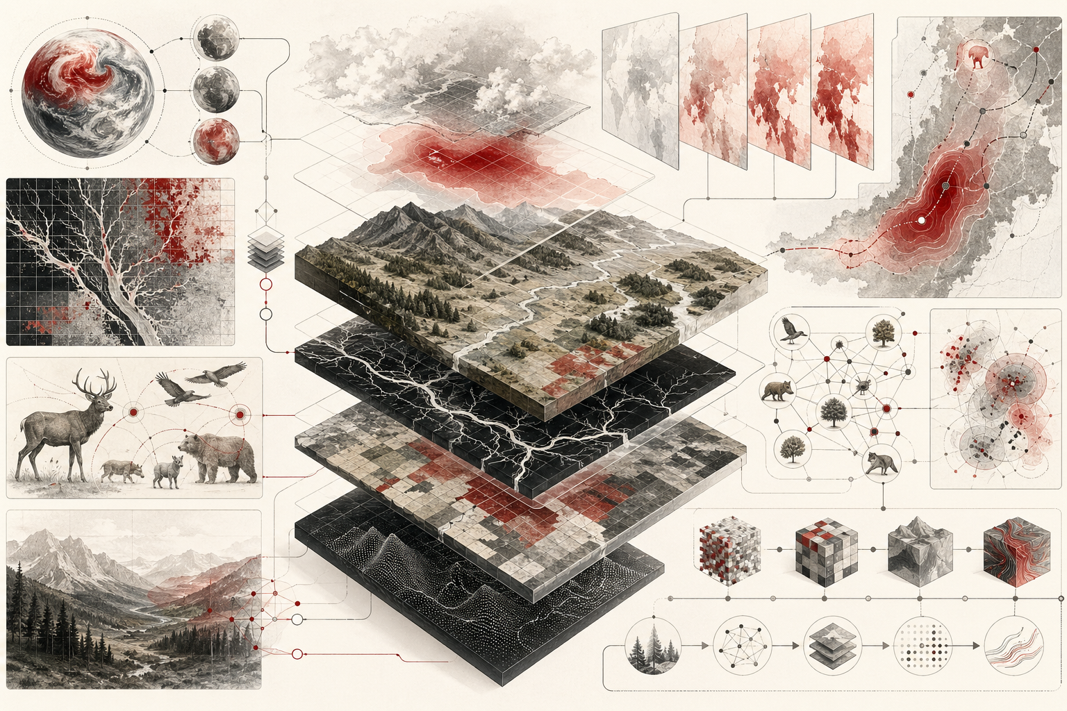
Computational ecology and environmental modeling give scientists a rigorous way to connect biological systems, environmental data, spatial processes, field observations, remote sensing, simulation, uncertainty, and reproducible workflows into models of how ecosystems function, change, recover, and respond to disturbance. Ecology has always been a science of interdependence. Computational ecology extends that tradition by using mathematical models, statistical inference, spatial data, simulations, scenario analysis, and environmental data systems to study living systems across scales.

This article introduces computational ecology and environmental modeling as a core methodological foundation for modern biology, conservation science, Earth-system research, restoration ecology, biodiversity science, environmental management, and sustainability analysis. It explains how ecological models help researchers examine species distributions, population dynamics, habitat suitability, disturbance regimes, hydrology, carbon fluxes, land-use change, climate stress, ecological restoration, environmental exposure, and coupled human-natural systems.

The article is written for ecologists, marine biologists, conservation biologists, environmental scientists, restoration ecologists, computational biologists, biodiversity researchers, geospatial analysts, data engineers, sustainability scientists, scientific software developers, and engineers. It emphasizes model assumptions, spatial scale, temporal scale, validation, environmental data quality, uncertainty, reproducibility, and responsible interpretation.

The article also extends the discussion into reproducible computational practice through Python and R examples, species-suitability modeling, patch-occupancy dynamics, environmental stress indices, simple hydrological runoff scaffolds, model-validation metrics, SQL-backed provenance, scenario analysis, and a linked full-stack GitHub repository containing Python, R, Julia, Fortran, Rust, Go, C, C++, SQL, notebooks, data files, validation notes, and reproducibility documentation.

Why computational ecology matters

Computational ecology matters because ecological systems are complex, dynamic, spatially structured, and increasingly exposed to rapid environmental change. Species move, populations fluctuate, disturbances propagate, climate variables shift, land cover changes, water flows, nutrients cycle, and human activities alter ecological conditions. These processes interact across scales, making purely verbal explanation insufficient.

Models help ecologists make assumptions explicit. A population model expresses how abundance changes. A habitat model expresses how environmental variables shape suitability. A hydrological model expresses how rainfall, soil, slope, and land cover affect runoff. A spatial model expresses how location and connectivity matter. A forecast model expresses how current data and uncertainty inform expectations about future states.

Computational ecology does not replace field ecology. It depends on field ecology. Observations, experiments, monitoring networks, environmental sensors, remote sensing, and ecological theory provide the empirical and conceptual foundation. Computation helps organize these inputs into structured analysis.

The central value of computational ecology is disciplined synthesis. It helps scientists move from fragmented observations to testable models, from local measurements to spatial inference, from historical patterns to scenario analysis, and from uncertainty to transparent decision support.

Back to top ↑

Ecological models as structured hypotheses

An ecological model is a structured hypothesis about how a living system works. It may be mathematical, statistical, spatial, mechanistic, agent-based, network-based, empirical, or hybrid. Its purpose is not simply to produce a number. Its purpose is to formalize relationships among organisms, environments, processes, and uncertainty.

A species-distribution model hypothesizes that occurrence depends on environmental conditions such as temperature, moisture, elevation, land cover, or habitat quality. A population model hypothesizes that abundance changes according to growth, carrying capacity, mortality, dispersal, or harvest. A food-web model hypothesizes interaction among species. A landscape model hypothesizes that patch connectivity affects persistence. A restoration model hypothesizes that intervention changes system trajectory.

The model’s assumptions determine what it can claim. If a model ignores dispersal, it may overestimate habitat occupancy. If a model ignores detection probability, it may confuse non-detection with absence. If a model uses coarse climate data, it may miss microclimatic refugia. If a model uses biased occurrence records, it may reproduce sampling effort rather than species ecology.

Computational ecology therefore requires interpretive discipline. Models should be treated as arguments, not oracles.

Back to top ↑

Environmental data as model infrastructure

Environmental models depend on data infrastructure. Ecological observations, biodiversity records, sensor measurements, satellite imagery, land-cover products, climate grids, soil maps, hydrological data, disturbance records, and management histories all shape model inputs. These data are not neutral; they reflect measurement systems, sampling design, resolution, coverage, uncertainty, and institutional practices.

A biodiversity occurrence record may reflect where a species was observed, but also where people looked. A satellite-derived vegetation index may reflect canopy greenness, but also atmospheric correction, sensor characteristics, cloud masking, viewing geometry, and spatial resolution. A climate raster may represent interpolated conditions across space, not a direct local measurement. A stream sensor may capture high-frequency data but only at one location.

This means environmental modeling begins with data criticism. What is the spatial resolution? What is the temporal resolution? What is the measurement method? What is missing? What is biased? What is interpolated? What is observed directly? What is derived? Which version? Which coordinate system? Which units?

Computational ecology becomes more trustworthy when data inputs remain traceable.

Back to top ↑

Spatial scale, temporal scale, and grain

Scale is one of the most important concepts in computational ecology. Ecological processes occur across space and time: microbial processes may shift over hours or millimeters, plant communities over years and meters, animal movement over days and kilometers, forest succession over decades, climate response over centuries, and watershed processes across entire regions.

Spatial grain refers to the size of the observational or modeling unit. Extent refers to the total area studied. Temporal grain refers to time step. Temporal extent refers to the period studied. These choices affect inference. A model built at one-kilometer resolution may miss habitat features visible at ten meters. A yearly model may miss seasonal dynamics. A daily hydrological model may miss storm pulses. A local population model may ignore regional dispersal.

Scale mismatches are common. Species occurrence data may be points, environmental data may be gridded, management units may be polygons, and ecological processes may occur across patch networks. Models must reconcile these structures carefully.

Good computational ecology documents scale choices and acknowledges what they make visible or invisible.

Back to top ↑

Species distribution and habitat suitability modeling

Species distribution modeling estimates where a species is likely to occur based on environmental conditions and known observations. Habitat suitability modeling estimates whether environmental conditions are favorable for a species or ecological community. These models are central in conservation planning, invasion biology, biodiversity monitoring, climate-change impact assessment, disease ecology, and ecological restoration.

A simple suitability model may combine temperature, precipitation, habitat quality, disturbance, and land cover. A statistical species-distribution model may relate presence records to environmental covariates. More advanced models may include detection probability, sampling bias, spatial autocorrelation, dispersal limits, biotic interactions, uncertainty, and future scenarios.

The central risk is overinterpretation. A suitability map is not a population census. A predicted distribution is not proof of presence. A model trained on biased observations may reproduce observer effort. A model projected into future climate may extrapolate beyond observed conditions. Environmental correlation does not prove causal mechanism.

Species-distribution modeling is strongest when paired with ecological knowledge, validation data, uncertainty estimates, and transparent assumptions.

Back to top ↑

Population dynamics and patch occupancy

Population models study how abundance changes through birth, death, immigration, emigration, resource limitation, disturbance, and environmental variability. Patch-occupancy models study whether habitat patches are occupied or unoccupied through colonization and extinction. These models are useful when abundance is difficult to measure but presence, absence, or detection data are available.

Patch dynamics are especially important in fragmented landscapes. A species may persist regionally even if local patches go extinct, provided colonization from other patches offsets losses. Connectivity, dispersal, habitat quality, disturbance, and matrix conditions affect persistence. A restoration project may improve habitat quality but fail if connectivity remains poor.

A simple occupancy model can represent patch state over time. Colonization probability increases the chance that empty patches become occupied. Extinction probability increases the chance that occupied patches become empty. Habitat quality may reduce extinction or increase colonization. Disturbance may do the opposite.

Patch models clarify ecological logic: persistence is not only about local habitat. It is also about landscape structure and movement.

Back to top ↑

Ecosystem processes, fluxes, and environmental drivers

Environmental modeling often focuses on processes and fluxes: water movement, carbon exchange, nutrient cycling, sediment transport, energy balance, evapotranspiration, primary production, decomposition, runoff, soil moisture, and greenhouse-gas exchange. These processes connect ecological systems to Earth systems.

A simple runoff model may estimate how precipitation, soil infiltration, land cover, and slope affect water movement. A carbon-flux model may relate photosynthesis, respiration, temperature, moisture, and vegetation structure. A nutrient model may track inputs, uptake, transformation, retention, and export. A disturbance model may represent fire, flood, drought, disease, or human land-use change.

These models are useful because ecological response often depends on physical conditions. A wetland plant community depends on hydrology. A stream ecosystem depends on flow and temperature. A forest carbon budget depends on climate, disturbance, age structure, and productivity. A coastal ecosystem depends on salinity, temperature, sea level, sediment, and storm exposure.

Computational ecology is therefore often interdisciplinary by necessity. It links biology with hydrology, climatology, geomorphology, soil science, remote sensing, geospatial analysis, and environmental engineering.

Back to top ↑

Remote sensing and Earth observation

Remote sensing has transformed environmental modeling because it provides repeated observations across large spatial extents. Satellite and airborne data can support vegetation monitoring, land-cover classification, fire detection, surface temperature mapping, snow and ice analysis, water quality assessment, coastal monitoring, drought assessment, and habitat mapping.

Remote sensing is not a substitute for field data. It measures reflected radiation, emitted energy, or sensor-derived signals that must be interpreted in context. Vegetation indices may indicate greenness, but not necessarily species composition. Land-cover classifications may simplify heterogeneous landscapes. Cloud cover, sensor calibration, atmospheric conditions, spatial resolution, and temporal frequency affect data quality.

The strength of remote sensing is scale. It allows environmental models to incorporate spatially extensive and repeated observations. The weakness is interpretation. Modelers must connect remote-sensing variables to ecological mechanisms and validate them against ground observations where possible.

In computational ecology, remote sensing is most powerful when integrated with field data, biodiversity records, sensor networks, ecological models, and uncertainty analysis.

Back to top ↑

Scenario analysis, climate stress, and land-use change

Environmental models often ask “what happens if?” What happens if temperature rises? What happens if precipitation declines? What happens if land cover changes? What happens if restoration improves habitat quality? What happens if disturbance frequency increases? What happens if connectivity improves? What happens if invasive species spread?

Scenario analysis explores plausible futures under different assumptions. It does not predict one certain future. It compares structured possibilities. A climate-stress scenario may increase temperature and reduce water availability. A restoration scenario may improve habitat quality. A disturbance scenario may increase mortality or reduce occupancy. A land-use scenario may reduce connectivity.

Scenario models are useful for planning because ecological decisions are made under uncertainty. Conservation, restoration, water management, infrastructure planning, biodiversity monitoring, and climate adaptation all require evaluating tradeoffs before outcomes are fully known.

The key requirement is transparency. Scenarios should be clearly named, parameterized, documented, and interpreted as conditional: if these assumptions hold, these model outcomes follow.

Back to top ↑

Uncertainty, validation, and forecasting

Ecological models contain uncertainty from many sources: measurement error, sampling bias, missing data, model structure, parameter uncertainty, climate variability, stochastic processes, spatial resolution, detection probability, and future human decisions. Computational ecology is strongest when it makes uncertainty visible.

Validation compares model outputs with independent observations or withheld data. A species-distribution model may be evaluated against test occurrence records. A population model may be compared against monitoring data. A hydrological model may be compared against streamflow observations. A forecast may be scored against future observations when they become available.

Ecological forecasting adds time pressure. Instead of only explaining past patterns, forecasting attempts to predict future ecological states in real time or near real time. Forecasts should include uncertainty intervals, update as new data arrive, and be evaluated against observations.

Forecasting shifts ecology toward a more iterative science: model, predict, observe, score, update, and learn.

Back to top ↑

Reproducibility, provenance, and open models

Computational ecology depends on reproducibility because models can be complex and consequential. A map, forecast, or scenario result should be traceable to data inputs, parameter settings, scripts, model version, coordinate system, units, assumptions, and outputs. Without provenance, ecological modeling becomes difficult to audit.

A reproducible project should include raw or source data references, processed data, scripts, documentation, model assumptions, validation reports, figures, and outputs. It should distinguish observed data from derived variables, parameters from outputs, and exploratory notebooks from production scripts. Version control and structured repositories help preserve this record.

Open models and open data are especially valuable in environmental science because ecological decisions often affect public goods: biodiversity, water, land, climate resilience, species protection, and community risk. Transparency supports review, reuse, accountability, and collaboration.

Reproducibility is not merely a technical preference. It is part of scientific responsibility.

Back to top ↑

Mathematical lens: computational ecology

Several mathematical ideas connect computational ecology and environmental modeling. These expressions do not replace field observation, ecological interpretation, Indigenous and local knowledge, or environmental judgment. They help clarify how population change, habitat suitability, environmental stress, runoff, prediction error, and scenario assumptions can be represented formally.

Logistic growth

Patch occupancy

Habitat suitability

Environmental stress index

Runoff scaffold

Root mean squared error

Mean absolute error

Scenario output

Back to top ↑

Python and R workflows

The following examples are compact article-level workflows. The full GitHub repository expands them into richer full-stack implementations with SQL provenance, cross-language validation, environmental scenario tables, patch dynamics, habitat suitability, runoff scaffolds, uncertainty summaries, and reproducible documentation.

Python example: habitat suitability model

import math
import pandas as pd

sites = pd.DataFrame(
    {
        "site_id": ["site_A", "site_B", "site_C", "site_D"],
        "temperature_c": [16.2, 22.5, 28.1, 19.4],
        "precipitation_mm": [820, 640, 410, 910],
        "habitat_quality": [0.82, 0.64, 0.31, 0.76],
        "disturbance": [0.18, 0.35, 0.72, 0.21],
    }
)

def logistic(value: float) -> float:
    return 1 / (1 + math.exp(-value))

def habitat_suitability(row) -> float:
    linear_score = (
        -2.0
        + 0.05 * row["temperature_c"]
        + 0.0015 * row["precipitation_mm"]
        + 2.4 * row["habitat_quality"]
        - 2.0 * row["disturbance"]
    )
    return logistic(linear_score)

sites["suitability"] = sites.apply(habitat_suitability, axis=1)

print(sites.round(4).to_string(index=False))

Python example: patch occupancy dynamics

import pandas as pd

def simulate_patch_occupancy(
    initial_occupancy: float,
    colonization: float,
    extinction: float,
    steps: int,
) -> pd.DataFrame:
    """Simulate simple regional patch occupancy."""
    occupancy = initial_occupancy
    rows = []

    for step in range(steps + 1):
        rows.append({"step": step, "occupancy": occupancy})

        occupancy = occupancy * (1 - extinction) + (1 - occupancy) * colonization
        occupancy = min(max(occupancy, 0.0), 1.0)

    return pd.DataFrame(rows)

baseline = simulate_patch_occupancy(
    initial_occupancy=0.42,
    colonization=0.12,
    extinction=0.08,
    steps=25,
)

print(baseline.tail().round(4).to_string(index=False))

Python example: climate-stress scenario analysis

import pandas as pd

scenarios = pd.DataFrame(
    {
        "scenario": ["baseline", "warming", "drying", "restoration"],
        "temperature_anomaly": [0.0, 2.5, 1.5, 1.5],
        "water_deficit": [0.15, 0.25, 0.45, 0.22],
        "disturbance": [0.25, 0.35, 0.40, 0.18],
        "habitat_gain": [0.00, 0.00, 0.00, 0.20],
    }
)

scenarios["stress_index"] = (
    0.40 * scenarios["temperature_anomaly"]
    + 1.50 * scenarios["water_deficit"]
    + 1.20 * scenarios["disturbance"]
    - 1.00 * scenarios["habitat_gain"]
)

scenarios["relative_resilience"] = 1 / (1 + scenarios["stress_index"])

print(scenarios.round(4).to_string(index=False))

Python example: simple runoff scaffold

import pandas as pd

grid = pd.DataFrame(
    {
        "cell_id": ["cell_01", "cell_02", "cell_03", "cell_04"],
        "precipitation_mm": [42, 55, 38, 61],
        "infiltration_fraction": [0.62, 0.48, 0.72, 0.35],
        "runoff_coefficient": [0.30, 0.42, 0.22, 0.58],
    }
)

grid["runoff_mm"] = (
    grid["precipitation_mm"]
    * (1 - grid["infiltration_fraction"])
    * grid["runoff_coefficient"]
)

print(grid.round(4).to_string(index=False))

Python example: model validation metrics

import math
import pandas as pd

validation = pd.DataFrame(
    {
        "site_id": ["site_A", "site_B", "site_C", "site_D", "site_E"],
        "observed_abundance": [18, 12, 4, 15, 9],
        "predicted_abundance": [16.5, 13.1, 5.2, 12.7, 8.4],
    }
)

errors = validation["observed_abundance"] - validation["predicted_abundance"]

rmse = math.sqrt((errors ** 2).mean())
mae = errors.abs().mean()
bias = errors.mean()

metrics = pd.DataFrame(
    {
        "metric": ["RMSE", "MAE", "Bias"],
        "value": [rmse, mae, bias],
    }
)

print(metrics.round(4).to_string(index=False))

R example: habitat suitability cross-check

# Compact R cross-check for habitat suitability.

sites <- data.frame(
  site_id = c("site_A", "site_B", "site_C", "site_D"),
  temperature_c = c(16.2, 22.5, 28.1, 19.4),
  precipitation_mm = c(820, 640, 410, 910),
  habitat_quality = c(0.82, 0.64, 0.31, 0.76),
  disturbance = c(0.18, 0.35, 0.72, 0.21)
)

logistic <- function(x) {
  1 / (1 + exp(-x))
}

sites$suitability <- logistic(
  -2.0 +
    0.05 * sites$temperature_c +
    0.0015 * sites$precipitation_mm +
    2.4 * sites$habitat_quality -
    2.0 * sites$disturbance
)

print(round(sites, 4))

Back to top ↑

GitHub repository

The article body includes compact Python and R examples so the scientific argument remains readable. The full repository expands those examples into a rigorous workflow for computational ecology and environmental modeling, including habitat suitability, patch occupancy, climate-stress scenarios, runoff scaffolds, validation metrics, environmental grids, scenario tables, provenance records, SQL audit structures, notebook documentation, cross-language validation helpers, and full-stack scientific-computing examples across Python, R, Julia, Fortran, Rust, Go, C, C++, SQL, and notebooks.

Back to top ↑

Limits, ethics, and responsible interpretation

Computational ecology can support powerful decisions, but models can also mislead. A habitat map can create a false sense of precision. A forecast can hide structural uncertainty. A scenario can appear inevitable when it is only conditional. A biodiversity model can reproduce sampling bias. A remote-sensing index can be overinterpreted. A model trained in one region can fail elsewhere.

Ethics matter because environmental models often influence land, water, species, communities, and policy. Species-location data can expose vulnerable populations to harm. Conservation models may affect Indigenous lands and local livelihoods. Climate-risk maps can influence insurance, infrastructure, investment, and public planning. Restoration models can prioritize some places over others. Environmental justice requires attention to who benefits, who bears risk, and whose knowledge is included.

Responsible modeling requires transparency, validation, uncertainty communication, community context, and humility. Models should support ecological judgment, not replace it.

Back to top ↑

Why computational environmental modeling matters

Computational environmental modeling matters because ecological change is accelerating. Climate change, habitat loss, invasive species, pollution, land-use change, water stress, biodiversity decline, and disturbance regimes are reshaping living systems faster than many institutions can respond. Models help organize evidence under uncertainty.

They allow scientists to compare scenarios, identify vulnerabilities, test mechanisms, design monitoring systems, evaluate restoration options, and communicate risks. They also help connect local observations to regional and global processes.

The deeper value is not prediction alone. It is structured accountability. A model makes assumptions visible. It can be tested, revised, challenged, and improved. In an era of ecological uncertainty, that transparency is essential.

Back to top ↑

Conclusion

Computational ecology and environmental modeling provide a rigorous framework for studying living systems in a changing world. They connect ecological theory, environmental data, spatial analysis, remote sensing, field observations, simulation, uncertainty, and reproducible workflows into structured scientific evidence.

The strongest models are not the most complicated. They are the clearest about their purpose, assumptions, inputs, scale, validation, uncertainty, and interpretation. They help ecologists ask better questions, compare plausible futures, identify mechanisms, and communicate evidence responsibly.

Used well, computational ecology does not distance biology from the living world. It helps make ecological interdependence more visible, testable, and accountable.

Back to top ↑

Related articles

• Biology
• Ecology and the Interdependence of Life
• Restoration Ecology and the Repair of Living Systems
• Mathematical Biology and the Logic of Living Systems
• Differential Equations in Population and Physiological Modeling
• Nonlinearity, Feedback, and Biological Regulation
• Networks, Systems, and Biological Complexity
• Probability, Variation, and Biological Inference
• Statistics, Uncertainty, and Measurement in Biology
• Data, Measurement, and Reproducibility in the Life Sciences
• Python for Biological Modeling and Automation

Further reading

• NSF NEON (n.d.) Open Data to Understand our Ecosystems. Available at: https://www.neonscience.org/data
• Ecological Forecasting Initiative and NEON (n.d.) NEON Ecological Forecasting Challenge. Available at: https://www.neonscience.org/efi-rcn-neon-ecological-forecasting-challenge
• NASA Earthdata (2026) Your Gateway to NASA Earth Observation Data. Available at: https://www.earthdata.nasa.gov/
• GBIF (n.d.) What is GBIF? Available at: https://www.gbif.org/what-is-gbif
• CSDMS (n.d.) Best Practices for Software Development. Available at: https://csdms.colorado.edu/wiki/CSDMS_Best_Practices_for_Software_Development
• NOAA Climate.gov (n.d.) Maps & Data. Available at: https://www.climate.gov/maps-data
• Copernicus Climate Data Store (n.d.) Climate Data Store. Available at: https://cds.climate.copernicus.eu/
• USGS (n.d.) Landsat Missions. Available at: https://www.usgs.gov/landsat-missions
• QGIS Project (n.d.) QGIS Documentation. Available at: https://docs.qgis.org/
• R Core Team (n.d.) The R Project for Statistical Computing. Available at: https://www.r-project.org/

References

• CSDMS (n.d.) Best Practices for Software Development. Available at: https://csdms.colorado.edu/wiki/CSDMS_Best_Practices_for_Software_Development
• Copernicus Climate Data Store (n.d.) Climate Data Store. Available at: https://cds.climate.copernicus.eu/
• Ecological Forecasting Initiative and NEON (n.d.) NEON Ecological Forecasting Challenge. Available at: https://www.neonscience.org/efi-rcn-neon-ecological-forecasting-challenge
• GBIF (n.d.) What is GBIF? Available at: https://www.gbif.org/what-is-gbif
• NASA Earthdata (2026) Your Gateway to NASA Earth Observation Data. Available at: https://www.earthdata.nasa.gov/
• NOAA Climate.gov (n.d.) Maps & Data. Available at: https://www.climate.gov/maps-data
• NSF NEON (n.d.) Open Data to Understand our Ecosystems. Available at: https://www.neonscience.org/data
• QGIS Project (n.d.) QGIS Documentation. Available at: https://docs.qgis.org/
• R Core Team (n.d.) The R Project for Statistical Computing. Available at: https://www.r-project.org/
• USGS (n.d.) Landsat Missions. Available at: https://www.usgs.gov/landsat-missions

Back to top ↑