
Last Updated August 4, 2026
Statistics, uncertainty, and measurement in biology examine how living systems become scientific evidence through measurement design, calibrated instruments, sampling, replication, uncertainty quantification, statistical modeling, and reproducible analysis. Biology studies organisms, cells, molecules, populations, ecosystems, tissues, biomarkers, genomes, images, and environmental signals that vary across time, space, lineage, condition, and scale. Because living systems are variable and measurements are never perfectly exact, biological knowledge depends on disciplined methods for distinguishing biological signal, measurement noise, sampling variation, experimental error, and uncertainty about mechanism.
This article introduces statistics and measurement as foundations of modern biological inference. It explains why biological measurement is not merely the act of recording numbers, but a structured process involving definitions, units, instruments, calibration, detection limits, uncertainty budgets, biological replication, technical replication, variance components, quality control, experimental design, data provenance, and model interpretation. It also explains why statistical reasoning is essential for deciding what biological measurements mean.
Main Library
Publications
Article Map
Biology
Related Topic
Mathematical Modeling
Related Topic
Environmental Science
Related Topic
Chemistry
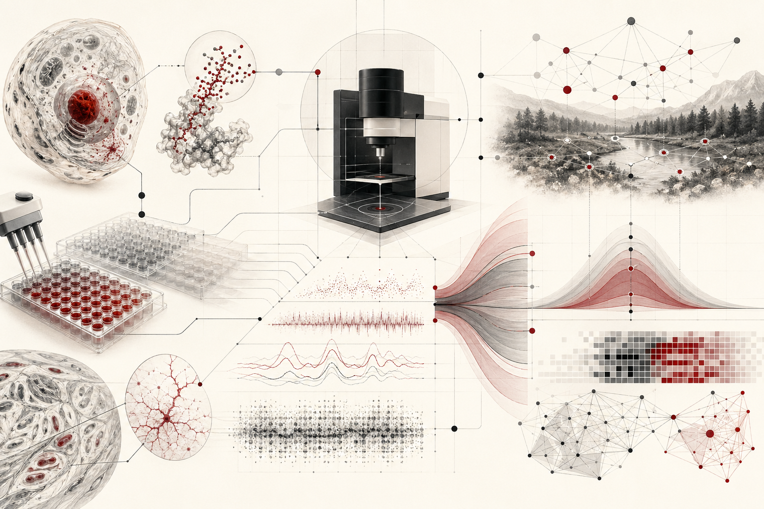
The article is written for biologists, ecologists, marine biologists, biomedical researchers, biotechnology scientists, epidemiologists, computational biologists, environmental scientists, engineers, metrologists, data scientists, and scientific readers who need a rigorous but usable framework for measurement and uncertainty in biological research. It treats statistics not as a post hoc add-on to biology, but as part of the architecture through which biological evidence becomes reliable.
The article also extends the discussion into reproducible computational practice through uncertainty budgets, measurement-error simulation, calibration curves, variance decomposition, confidence intervals, bootstrap intervals, assay quality control, mixed-effects scaffolds, error propagation, R workflows, Python workflows, SQL provenance structures, and a linked full-stack GitHub repository containing Python, R, Julia, Fortran, Rust, Go, C, C++, SQL, notebooks, data files, validation notes, and reproducibility documentation.
Updated August 2026: This edition expands the article to include metrological traceability, commutability, fitness for purpose, study design, precision-based sample planning, missingness and censoring, effect sizes and estimands, multiplicity, hierarchical and causal models, omics and imaging measurement, AI-enabled measurement systems, current reporting guidance, and decision-focused uncertainty. It also reflects JCGM GUM-5:2026, FDA’s 2026 biomarker-method guidance, CONSORT 2025, TRIPOD+AI, ARRIVE 2.0, FAIR data principles, and NIH’s renewed replication and reproducibility initiatives.
Why measurement is central to biology
Biology becomes scientific when living systems can be observed, compared, measured, modeled, and tested. Measurement is therefore not a minor technical step between observation and interpretation. It is one of the central acts through which biological phenomena become evidence. A cell count, gene-expression value, enzyme velocity, body temperature, microbial abundance, pollutant concentration, species richness estimate, survival rate, biomarker level, image-derived cell area, or oxygen measurement is not merely a number. It is the result of a measurement process.
That process matters because biological systems vary. A measured value may reflect the organism, sample, instrument, operator, assay, environment, time of day, calibration state, sample handling, batch effect, statistical model, or computational pipeline. If the measurement process is poorly understood, the biological interpretation may be weak even when the numerical output looks precise.
Statistics enters biology because measurement alone is not enough. Once measurements exist, scientists must ask how much they vary, how uncertain they are, whether differences are meaningful, whether estimates generalize beyond the sample, whether instruments were calibrated, whether variation is biological or technical, and whether the analysis matches the design. Measurement produces data; statistics helps determine what those data can responsibly support.
The purpose of measurement in biology is not only to produce numbers. It is to make claims about living systems more precise, testable, comparable, and reproducible.
Measurement also determines what a discipline is able to see. A biological process may remain scientifically invisible when no reliable measurand, sampling frame, assay, reference procedure, or computational representation exists. New instruments do more than increase precision: they can create new biological objects of study. Flow cytometry made heterogeneous cell populations measurable at scale. Sequencing converted genomes and transcriptomes into analyzable records. Automated microscopy turned morphology into high-dimensional data. Environmental sensors and molecular detection expanded the temporal and spatial reach of field biology. Each advance, however, also introduced new transformations between living phenomenon and reported result.
This is why the quality of biological evidence cannot be judged from the final statistical output alone. The inferential chain begins earlier: defining the biological question, identifying the target population or system, specifying the measurand, choosing the experimental unit, designing sampling, controlling pre-analytical variation, validating the measurement procedure, and documenting the transformations that produce the analytical dataset. A narrow focus on significance tests can conceal failure anywhere along this chain.
In August 2026, measurement science is also becoming more explicit about the relationship between uncertainty and use. The Joint Committee for Guides in Metrology has expanded the GUM family with JCGM GUM-5:2026, a collection of worked examples for evaluating and expressing measurement uncertainty. In biomedical regulation, the U.S. Food and Drug Administration issued final 2026 guidance on bioanalytical method validation for biomarkers, while NIH has renewed its institutional focus on replication and reproducibility. These developments reinforce a common principle: a number becomes evidence only when its definition, traceability, uncertainty, and intended use are visible.
Measurands, Targets, and Decision Context
A biological measurement begins with a target concept, but the target concept is not always identical to the operational measurand. “Inflammation,” “ecosystem health,” “cell viability,” “viral load,” “treatment response,” and “biodiversity” are broad constructs. A measurement procedure captures a defined indicator under specified conditions. The gap between construct and operational measure is a source of uncertainty that cannot be solved by instrument calibration alone.
A useful measurement specification should identify at least six elements: the biological system, the quantity or property, the unit or category, the temporal and spatial conditions, the measurement procedure, and the intended use. For example, “dissolved oxygen” may mean milligrams per litre at a specified depth, temperature, salinity, sensor type, calibration state, and sampling interval. “Gene expression” may mean normalized transcript abundance for a defined transcript set, tissue, extraction protocol, sequencing platform, and computational pipeline. “Diagnostic sensitivity” depends on the target condition, reference standard, threshold, population, and handling of indeterminate results.
Intended use matters because acceptable uncertainty is contextual. A rough field screen, a discovery assay, a clinical diagnostic, a release specification, and a regulatory monitoring system do not require the same evidence. A method can be fit for exploratory ranking but unfit for individual treatment decisions. A model may be suitable for population surveillance but unsafe for person-level classification. Measurement quality should therefore be evaluated against the decision that the result is expected to support.
This perspective changes validation from a ritual into an argument. Validation asks whether a measurement procedure is sufficiently reliable for a specified purpose under defined conditions. It does not certify a method for every sample, laboratory, population, software version, or future use.
Measurement as a biological and instrumental process
Every biological measurement has two sides. One side is biological: what is being measured? The other side is instrumental or procedural: how is it being measured? A glucose concentration, chlorophyll fluorescence value, DNA copy number, species count, viral load, enzyme rate, dissolved oxygen reading, or cell morphology summary depends on both.
The biological side requires defining the measurand: the quantity intended to be measured. In biology, the measurand can be difficult to define because living systems change. A biomarker may fluctuate over hours. A population may move. A microbial community may shift during storage. A tissue sample may degrade. A fluorescence signal may represent both biological abundance and technical background. A field measurement may depend on season, weather, depth, or habitat structure.
The instrumental side includes sampling, preparation, calibration, instrument response, detection limit, operator procedure, data processing, and computational transformation. A sequencing read count is not simply “gene expression.” It is the result of extraction, library preparation, sequencing, alignment, filtering, normalization, and statistical modeling. A satellite-derived vegetation index is not simply “plant health.” It is a measurement product shaped by sensor physics, atmospheric correction, spectral response, spatial resolution, and ecological interpretation.
Good biological measurement therefore requires traceability from biological question to measurement workflow. The stronger the chain between phenomenon, method, data, and inference, the more reliable the biological claim.
Measurement systems also include classification rules. A histopathology grade, disease status, cell phenotype, habitat class, behavioral category, or algorithmic label may not be expressed on a continuous physical scale, yet it is still produced by a measurement process. The relevant questions include how categories are defined, whether observers agree, what reference standard is used, whether borderline cases are handled consistently, and whether the classification remains valid across populations, instruments, sites, and time.
The measurand must therefore include conditions. “Protein concentration” is incomplete if concentration depends on specimen matrix, extraction protocol, molecular form, temperature, timing, or assay specificity. “Species abundance” is incomplete if the observation process ignores detectability, sampled area, life stage, season, or taxonomic resolution. “Tumor area” is incomplete if segmentation conventions and image magnification are unspecified. Defining the measurand is a scientific act because it determines what the result claims to represent.
Metrological Traceability, Reference Systems, and Commutability
Metrological traceability is the property of a measurement result whereby it can be related to a reference through a documented, unbroken chain of calibrations, each contributing to measurement uncertainty. Traceability belongs to the result, not merely to the instrument or laboratory. Saying that an instrument is “NIST traceable” is incomplete unless the reference, calibration chain, uncertainty contributions, measurement procedure, and conditions of use are documented.
Biology complicates traceability because many measurands are structurally heterogeneous, method-defined, or unstable. A protein may exist in multiple isoforms. A cell population may lack a single reference material. A clinical biomarker may be matrix-dependent. A microbial community has no simple SI realization. A sequencing count is generated by an analytical pipeline rather than direct comparison with a physical unit. In such cases, traceability may lead to a certified reference material, reference measurement procedure, consensus standard, calibration hierarchy, or operationally defined reference rather than directly to an SI unit.
Commutability is critical in laboratory medicine and other matrix-sensitive measurements. A reference material is commutable when it behaves like real samples across relevant measurement procedures. A non-commutable control can produce reassuring calibration results while failing to represent patient specimens, environmental samples, or biological matrices. Reference material quality therefore includes matrix match, stability, homogeneity, characterization, and fitness for purpose.
Traceability also has a computational form. Software versions, reference databases, annotation releases, model weights, preprocessing parameters, and random seeds can function as links in the measurement chain. A variant call cannot be reproduced if the genome build and caller version are unknown. An image-derived phenotype is not traceable if segmentation settings are hidden. A model-generated score requires provenance for training data, feature extraction, threshold selection, and deployment version.
The practical goal is not to force every biological quantity into an inappropriate physical-metrology template. It is to make the reference system and transformation chain explicit enough that results can be compared, audited, reproduced, and interpreted within their limits.
Accuracy, precision, bias, and uncertainty
Accuracy, precision, bias, and uncertainty are related but distinct ideas. Precision concerns repeatability: how close repeated measurements are to one another. Accuracy concerns closeness to the intended or accepted value. Bias is systematic deviation. Uncertainty characterizes the range or dispersion of values that could reasonably be attributed to the measurand.
Biological researchers often confuse these concepts. A method can be precise but biased. Repeated assay readings may cluster tightly around the wrong value if calibration is poor. A method can be unbiased but imprecise. Measurements may average correctly over many trials while individual readings vary widely. A result can have small statistical standard error while still being biased by poor sampling or flawed design.
Uncertainty is especially important because it is more honest than false exactness. A measurement reported without uncertainty may imply more confidence than the method deserves. In biology, uncertainty can arise from instrument resolution, calibration, sample preparation, biological heterogeneity, operator differences, environmental variability, model assumptions, and computational processing.
Reporting uncertainty does not weaken a result. It strengthens the result by making the reliability of the measurement visible. A biological claim that includes uncertainty can be evaluated, compared, propagated through models, and improved.
Trueness and accuracy are sometimes used differently across technical communities. In metrology, accuracy is a qualitative concept rather than a numerical quantity, while bias can be estimated from repeated comparisons with a reference. In biological practice, researchers should state the operational definition they are using instead of assuming the terms are self-explanatory. The same caution applies to repeatability, intermediate precision, reproducibility, reliability, agreement, sensitivity, specificity, and robustness.
Uncertainty also has layers. Measurement uncertainty concerns the values reasonably attributable to a measurand under a specified model. Sampling uncertainty concerns which biological units were observed. Model uncertainty concerns the analytical representation. Decision uncertainty concerns whether the evidence is sufficient for an action. These layers overlap but should not be collapsed into one confidence interval. A narrow interval around a biased or poorly defined quantity is not reliable evidence.
Validity, Reliability, Agreement, and Fitness for Purpose
Validity asks whether a measurement captures the phenomenon it is intended to represent. Reliability asks whether repeated measurements distinguish biological units consistently. Agreement asks how close measurements are in the units that matter. These questions are related but not interchangeable.
A high correlation does not demonstrate agreement. Two instruments can track one another closely while one is systematically higher. A high intraclass correlation can occur when between-subject variation is large even if repeated measurements differ enough to matter clinically. A low coefficient of variation can look impressive for a large-valued quantity while absolute error remains unacceptable. Method comparison should therefore include difference plots, bias estimates, limits of agreement, concentration-dependent error, heteroscedasticity, and predefined acceptability criteria.
Construct validity is especially important for complex biological indicators. A composite “health score,” “stress index,” “cell state,” or “ecosystem condition” may combine multiple variables, weights, transformations, and thresholds. Its numerical precision does not establish that the construct is biologically coherent. Validation may require convergent evidence, known-group comparisons, response to perturbation, predictive performance, mechanistic plausibility, and stability across contexts.
Fitness for purpose integrates these concerns. The same assay may be adequate for screening but not quantification, adequate for group comparison but not individual classification, or adequate within one range but unreliable near a decision threshold. Researchers should define performance requirements before seeing the data whenever possible. Post hoc standards invite self-confirming validation.
| Question | Relevant concept | Common mistake |
|---|---|---|
| Does the result represent the intended biological property? | Validity | Assuming a convenient proxy is the construct itself. |
| Are repeated measurements consistent across units or raters? | Reliability | Using correlation alone. |
| Are measurements close enough in meaningful units? | Agreement | Ignoring systematic and proportional bias. |
| Can the method support the intended decision? | Fitness for purpose | Generalizing validation beyond the tested context. |
Biological variation and measurement error
Biological variation and measurement error should not be treated as the same thing. Biological variation is real difference among biological units or states. Measurement error is uncertainty introduced by the measurement process. Both can appear as variation in data, but they have different meanings.
For example, variation in cell size across a tissue sample may reflect real differences in cell cycle stage, differentiation state, or local environment. Variation in measured cell size may also reflect segmentation error, imaging resolution, staining differences, or threshold choices. Variation in blood pressure may reflect physiological fluctuation, posture, stress, time of day, cuff placement, or instrument calibration. Variation in ecological abundance may reflect true patchiness, imperfect detection, sampling effort, or observer differences.
The statistical challenge is to separate sources of variation when possible. Variance components, mixed-effects models, repeated-measures designs, technical replicates, calibration standards, blanks, controls, and hierarchical models all help distinguish biological signal from measurement process. Without this distinction, researchers may overstate confidence, miss real biological heterogeneity, or treat measurement artifacts as biological findings.
This distinction is especially important in high-throughput biology. Batch effects in sequencing, plate effects in assays, scanner effects in imaging, and site effects in field data can dominate biological interpretation if not identified and controlled.
Measurement error can attenuate associations, inflate residual variation, distort classification, create regression dilution, and change estimated treatment effects. Misclassification can be differential or non-differential with respect to exposure or outcome, and those patterns can bias results in different directions. Corrective methods—such as regression calibration, simulation-extrapolation, latent-variable models, validation subsamples, repeated measurements, and Bayesian measurement models—require information about the error process. They cannot recover what was never measured or documented.
Biological heterogeneity should not automatically be “controlled away.” Variation by sex, age, genotype, developmental stage, microbial community, environment, tissue state, or prior exposure may be part of the phenomenon. The design problem is to distinguish nuisance variation from scientifically meaningful variation. That requires pre-specified biological reasoning rather than indiscriminate adjustment.
Replication: technical, biological, and experimental
Replication is essential to biological measurement, but different kinds of replication answer different questions. Technical replication measures repeatability of the procedure. Biological replication measures variation among independent biological units. Experimental replication tests whether a finding can recur under repeated study conditions. Confusing these forms of replication can seriously weaken inference.
Technical replicates are useful for estimating instrument or procedural variability. Multiple qPCR wells, repeated instrument readings, replicate assay wells from the same sample, or repeated image measurements can reveal measurement precision. But technical replicates are not equivalent to independent organisms, cultures, plots, patients, tanks, reefs, or ecosystems.
Biological replicates matter because biology varies across independent living units. If a study has many technical replicates but few biological replicates, it may estimate procedural precision well while failing to estimate biological variability. This can produce exaggerated confidence.
Good experimental design defines the experimental unit before data collection. Is the unit a cell, culture, animal, patient, plot, tank, reef, sample, field site, or batch? The answer determines what counts as independent evidence. Statistical analysis must respect this structure. Pseudoreplication occurs when non-independent observations are treated as independent; it remains one of the major threats to biological inference.
Independence is often the hidden issue. Thousands of cells from one animal do not become thousands of independent animals. Multiple images from one tissue section do not become independent specimens. Repeated water samples from one reach do not represent multiple rivers. The effective sample size is constrained by the level at which treatment, exposure, or biological variation operates. Hierarchical analysis can use lower-level observations without pretending that they create higher-level replication.
Replication should also be separated from reproducibility and robustness. A computational rerun reproduces an analysis from the same data and code. A repeat measurement evaluates procedural stability. An independent experiment evaluates whether a result recurs under newly generated data. A conceptual replication tests the underlying claim with different operationalizations. Robustness analysis asks whether conclusions survive reasonable alternative assumptions. Each strengthens evidence in a different way.
Study Design: Randomization, Blinding, Blocking, and Controls
Statistical validity begins with design. Randomization protects against systematic allocation differences and supports probabilistic inference. Blinding reduces differential treatment, measurement, and analysis. Blocking increases precision by grouping units that share important sources of variation. Controls define what change should be attributed to the intervention rather than time, handling, background signal, contamination, or instrument drift.
Randomization must occur at the correct level. If treatment is assigned by tank, cage, plate, field, classroom, or clinic, that cluster—not every observation within it—is the randomized unit. Restricted randomization, stratification, and blocking can improve balance, but the analysis must account for the procedure used. Convenience allocation, alternating assignment, or assigning treatments by plate column can create confounding that no later p-value repairs.
Blinding is not all-or-nothing. Investigators can blind intervention labels during imaging, sample preparation, outcome assessment, exclusion decisions, or statistical analysis even when treatment delivery cannot be blinded. Automated measurement is not automatically unbiased: algorithms can encode batch, site, demographic, or preprocessing differences. Masked file names and locked analysis scripts may be as important as blinded observers.
Negative controls reveal contamination and background. Positive controls show that the system can detect an expected signal. Vehicle controls distinguish treatment from delivery effects. Reference controls support comparability across batches. Process controls track extraction, amplification, staining, transport, or computational stages. Controls should be designed around failure modes rather than added mechanically.
Pre-specified exclusion criteria are part of measurement design. Excluding outliers, failed wells, low-quality images, or implausible field observations after reviewing outcomes can alter estimates and uncertainty. A defensible workflow records reasons, applies rules consistently, preserves raw data, and reports sensitivity analyses with and without disputed observations.
Sample Size, Power, Precision, and Information
Sample-size planning should begin with the estimand and decision, not a generic rule. A study may need to estimate a mean with a specified margin of error, detect a biologically meaningful contrast, quantify diagnostic sensitivity, estimate a variance component, validate a prediction model, or characterize rare adverse events. Each goal requires different information.
Statistical power is the probability of rejecting a null model under a specified alternative, design, variance, and analysis. It is not the probability that a significant result is true, and post hoc “observed power” adds little beyond the p-value. Planning assumptions should include effect size, biological variability, technical error, attrition, clustering, repeated measures, multiplicity, and the smallest effect that would change interpretation or action.
Precision-based planning is often more transparent than power alone. Researchers can define an acceptable confidence-interval width, uncertainty range, or prediction error. For diagnostic studies, precision may be required separately for sensitivity and specificity. For ecological occupancy, the number of sites and repeat visits jointly determine information. For mixed models, the number of higher-level clusters often matters more than the number of observations within each cluster.
More data do not automatically correct bias. Increasing technical replicates reduces uncertainty about one sample’s procedural mean but does not create new biological units. Expanding a biased convenience sample can produce a very narrow interval around the wrong population quantity. Information depends on representativeness, design, measurement quality, and independence as well as count.
Adaptive and sequential designs can use data efficiently, but they require pre-specified stopping and decision rules. Optional stopping, repeated significance testing, or undisclosed sample-size changes inflate error rates and undermine interpretation. Flexibility should be governed rather than hidden.
Missing Data, Censoring, Detection Limits, and Non-Detects
Missingness is part of the measurement process. Samples may be unavailable, degraded, lost, below detection, technically failed, excluded by quality control, or absent because an organism, patient, or site could not be observed. Treating every missing value as interchangeable discards information about why measurement failed.
Statistical discussions often distinguish data missing completely at random, missing at random conditional on observed variables, and missing not at random. These are modeling assumptions, not labels that can be read directly from the dataset. In biology, missingness is frequently informative: sicker patients may miss visits, low-abundance taxa may escape detection, fragile samples may fail processing, and extreme values may exceed instrument range.
A result below the limit of detection is not zero. Substituting zero, half the detection limit, or the detection limit itself can distort distributions, correlations, and trends. Better approaches depend on the question and data-generating process: censored likelihoods, interval reporting, multiple imputation, hurdle models, occupancy models, or sensitivity analysis. Limits of detection and quantification should be defined by a documented procedure and reported with the calibration range and matrix.
Indeterminate, invalid, and uninterpretable results also matter in diagnostic studies. Excluding them can make performance look better than practice. Transparent reporting should show how many occurred, why, in whom, and how alternative handling changes sensitivity, specificity, predictive values, and clinical consequences.
Missingness management begins operationally: redundant identifiers, sample tracking, audit trails, instrument alerts, reason codes, repeat-measurement rules, and preservation of raw outputs. Statistical methods cannot fully compensate for an undocumented measurement pathway.
Uncertainty budgets and error propagation
An uncertainty budget identifies the major sources of uncertainty in a measurement process and combines them into an overall uncertainty estimate. In biology, such sources may include instrument precision, calibration uncertainty, sample preparation variability, operator effects, environmental conditions, biological heterogeneity, reference-material uncertainty, dilution error, image-processing error, and model uncertainty.
The advantage of an uncertainty budget is that it makes uncertainty auditable. Rather than reporting a single number without context, a researcher can show how much uncertainty comes from each part of the workflow. This is useful in biotechnology, environmental monitoring, clinical assays, toxicology, ecological measurement, and laboratory quality systems.
Error propagation is needed when measured quantities are combined. If biomass is calculated from length and width, uncertainty in both measurements affects biomass uncertainty. If concentration is calculated from instrument response and calibration slope, uncertainty in both contributes to the final concentration. If an ecological index is calculated from multiple counts, uncertainty in sampling and detection affects the index.
Uncertainty propagation helps prevent false precision. A derived quantity cannot be more trustworthy than the measurements and assumptions used to produce it. In biological modeling, uncertainty should travel with the data.
Uncertainty components should be expressed on a common scale and accompanied by their evidence source. Type A evaluation uses statistical analysis of repeated observations. Type B evaluation uses other information such as calibration certificates, reference-material characterization, instrument specifications, prior validation, or expert knowledge. “Type B” does not mean subjective or inferior; it describes the method of evaluation.
Correlation among components matters. Temperature may affect both calibration and sample stability. One reagent lot may influence multiple analytes. Shared normalization can induce covariance across features. Root-sum-of-squares calculations that assume independence can understate or overstate uncertainty when common causes are important. Monte Carlo propagation is useful when models are nonlinear, distributions are asymmetric, thresholds are present, or covariance is complex.
An uncertainty budget should be proportional to the decision. Not every exploratory assay needs a national-metrology-level analysis, but consequential clinical, environmental, manufacturing, or regulatory measurements require explicit evidence that uncertainty is acceptable for use. JCGM GUM-1:2023 provides an updated introduction to these decisions, and GUM-5:2026 adds worked examples that help translate principles into practice.
Calibration, detection limits, and assay quality
Calibration connects instrument response to known reference values. Without calibration, measurements may be internally consistent but externally unreliable. Calibration curves are central in analytical chemistry, molecular assays, environmental monitoring, microscopy, flow cytometry, qPCR, ELISA, spectroscopy, sensor systems, and many biotechnology workflows.
Detection limits also matter. A measurement below the limit of detection should not be interpreted the same way as a true zero. In ecology, environmental DNA detection may depend on concentration, degradation, sampling volume, inhibitors, and assay sensitivity. In medicine, biomarker detection may depend on specimen handling, analytical sensitivity, and biological variability. In environmental monitoring, pollutant concentrations near detection limits require careful reporting.
Assay quality often involves precision, accuracy, linearity, dynamic range, limit of detection, limit of quantification, sensitivity, specificity, reproducibility, robustness, and interference testing. These are not bureaucratic details. They determine whether the measurement can support the claim being made.
For engineers and biotechnology researchers, assay quality is also a design problem. A biosensor, diagnostic test, fermentation monitor, imaging pipeline, or automated platform must be evaluated not only by whether it produces data, but by whether the data are reliable under expected conditions of use.
Calibration range should cover the values used for inference. Extrapolating beyond standards may produce implausible estimates even when the fitted line has a high coefficient of determination. Residual patterns, weighting, heteroscedasticity, replicate standards, blank behavior, carryover, dilution integrity, and matrix effects are often more informative than \(R^2\) alone.
Current regulatory guidance increasingly emphasizes lifecycle and context. FDA’s final Q2(R2) and Q14 guidances frame analytical validation and development as connected activities. Its April 2026 guidance on bioanalytical method validation for biomarkers addresses methods used to quantify biomarker concentrations in human samples supporting drug development. The regulatory details are context-specific, but the general scientific lesson is broad: validation characteristics, acceptance criteria, study samples, and documentation should be linked to intended use.
Quality control is not only a pass/fail gate. Control-chart patterns can reveal drift, shifts, increasing variability, reagent degradation, and operator changes. A run that technically passes all controls may still show a pattern requiring investigation. Conversely, overly narrow limits can generate repeated false alarms that encourage normalization of deviance.
Statistics as the language of measured life
Statistics gives measured biology its inferential structure. Descriptive statistics summarize data. Inferential statistics estimate population quantities from samples. Regression models quantify relationships. Mixed-effects models account for nested and repeated structures. Bayesian models update uncertainty. Time-series models analyze change. Multivariate models examine high-dimensional biological patterns. Survival models analyze time-to-event outcomes. Measurement-error models account for imperfect observations.
The key is that statistical methods must match biological design. A paired design should not be analyzed as independent groups. Repeated measures should not be treated as unrelated. Nested samples should not be flattened. Technical replicates should not be substituted for biological replication. Count data, proportions, censored values, compositional data, and spatially correlated data often require methods designed for those structures.
Statistics is therefore not a decoration added at the end of a study. It is part of measurement design. The question, sampling strategy, measurement workflow, replication structure, and statistical model should be planned together. When statistical analysis is delayed until after data collection, design weaknesses may already be irreversible.
The purpose of statistics in biology is not merely to produce p-values. It is to connect measurement, uncertainty, model, and biological interpretation.
Statistical models also determine the scale of the claim. Population-average and subject-specific effects can differ. Conditional and marginal estimates can answer different questions. A model for the mean may not describe variability, tail risk, or individual prediction. Researchers should state whether they seek explanation, description, prediction, screening, or decision support.
Effect estimates should be interpreted alongside measurement capability. An apparent change smaller than the method’s repeatability or long-term reproducibility may not be distinguishable from measurement variation. Conversely, a noisy method can obscure an important biological effect. Statistical power and measurement precision are therefore connected design parameters.
Estimands, Effect Sizes, and Interval-Based Inference
An estimand is the quantity a study seeks to estimate. It specifies the population, outcome, contrast, time horizon, and handling of events such as treatment switching, death, dropout, or rescue intervention. Clear estimands prevent a common problem: collecting data for one question and reporting an analysis that answers another.
Effect sizes describe magnitude. Depending on the design, they may include mean differences, standardized differences, risk differences, risk ratios, odds ratios, rate ratios, hazard ratios, correlation coefficients, variance explained, calibration slopes, or changes in prediction error. Biological interpretation should emphasize units and consequences. A standardized effect can aid comparison but may hide whether the underlying change is biologically or clinically important.
Intervals are often more informative than dichotomous thresholds. A confidence interval shows the range of parameter values compatible with the data and model at a specified confidence procedure. A Bayesian credible interval expresses posterior uncertainty under the model and prior. A prediction interval addresses future observations and is usually wider than an interval for the mean. An agreement interval addresses differences between methods. These intervals answer different questions.
Statistical compatibility is not practical equivalence. A wide interval that includes zero may also include effects large enough to matter. A narrow interval excluding zero may describe a trivial change. Equivalence and non-inferiority questions require predefined margins justified by biology, clinical relevance, measurement capability, and decision cost.
Uncertainty should follow the estimand through subgroup, sensitivity, and missing-data analyses. Reporting one favored estimate while hiding alternative defensible specifications creates a false sense of stability. A multiverse or specification-curve analysis can show how conclusions depend on analytic choices, but it should complement—not replace—a principled primary analysis.
P-values, Multiplicity, Selective Analysis, and Researcher Degrees of Freedom
A p-value is a probability calculated under a statistical model, typically describing how incompatible the observed data or a more extreme result would be with a specified null hypothesis. It is not the probability that the hypothesis is true, the probability that the result occurred by chance, or a measure of effect importance. Thresholds such as 0.05 are conventions, not biological laws.
Multiplicity arises when many outcomes, groups, time points, genes, taxa, models, thresholds, or hypotheses are examined. Without adjustment or hierarchical structure, the chance of at least one apparently unusual result increases. Family-wise error control, false-discovery-rate procedures, shrinkage, multilevel modeling, and pre-specified outcome families address different goals. In omics and imaging, multiplicity may involve millions of correlated features, making naive single-test reasoning untenable.
Selective reporting can be more damaging than multiplicity itself. Researchers may choose an outcome, transformation, covariate set, exclusion rule, subgroup, or stopping point after seeing the data. Each choice may be individually plausible while the unreported search process makes the final result look more certain than it is. Registered reports, preregistration, analysis plans, blinded analysis, and complete reporting reduce this distortion.
Exploratory analysis remains scientifically valuable. The problem is not exploration; it is presenting exploration as confirmatory evidence. Exploratory results should be labeled, accompanied by the search space and uncertainty, and tested in new data when the claim requires confirmation.
Measurement error interacts with multiplicity. No correction for multiple testing repairs systematic batch effects, contaminated controls, or mislabeled samples. Statistical safeguards operate downstream of measurement integrity.
Model Assumptions, Diagnostics, and Robustness
Every statistical model simplifies biology. Linear models assume a form for the mean and residual structure. Generalized models assume a response distribution and link. Survival models may assume proportional hazards. mixed-effects models assume a random-effect structure. Machine-learning models assume that training and deployment data are sufficiently related. The task is not to find an assumption-free method, but to make assumptions visible and test consequences.
Diagnostics should be tied to failure modes. Residual plots can reveal nonlinearity, heteroscedasticity, outliers, and dependence. Influence analysis can identify observations that dominate estimates. Calibration plots can show systematic prediction error. Posterior predictive checks can reveal whether a Bayesian model reproduces important features of the data. Spatial and temporal correlograms can detect dependence left in residuals.
Robustness analysis asks whether the scientific conclusion changes under reasonable alternatives. Examples include robust standard errors, transformation choices, alternative distributions, exclusion rules, missing-data assumptions, different priors, cluster definitions, lag structures, batch corrections, or measurement-error parameters. Robustness should focus on the decision-relevant conclusion rather than whether every coefficient remains below a threshold.
Data transformations deserve biological interpretation. Log transformation changes additive differences into multiplicative relationships. Normalization can remove library size or technical variation but may also remove biological signal. Standardization changes units and can obscure practical magnitude. Compositional transformations address relative data but alter the interpretation of coefficients. Each transformation belongs in the measurement model, not merely the software script.
Model fit is not model truth. A highly flexible model can interpolate a dataset while failing under new sites, batches, populations, seasons, or instruments. External validation and transportability are stronger tests than in-sample performance.
Hierarchical, Mixed-Effects, and Bayesian Measurement Models
Biological data are frequently hierarchical: technical replicates within samples, cells within tissues, tissues within organisms, organisms within cages, plots within landscapes, repeated visits within sites, and batches within laboratories. Hierarchical models represent this structure explicitly and allow uncertainty to be allocated across levels.
Mixed-effects models include fixed effects for contrasts of scientific interest and random effects for variation among sampled groups. They can estimate between-unit and within-unit variance, account for repeated measures, and avoid treating clustered observations as independent. Random-effects structure should reflect design and scientific goals; complex models can become unstable when the number of higher-level units is small.
Bayesian models combine likelihood, prior information, and hierarchical structure to produce posterior distributions. They are especially useful when measurement error is substantial, data are sparse, latent biological states are important, or information must be shared across related groups. Priors can regularize noisy estimates, but they must be justified and subjected to sensitivity analysis.
Latent-variable models separate an unobserved biological quantity from imperfect indicators. Occupancy models distinguish species presence from detection. Item-response models distinguish latent traits from responses. Measurement-error models distinguish true exposure from observed exposure. State-space models distinguish ecological or physiological process from observation noise. These models make the observation process part of inference rather than pretending that measured values equal biological truth.
Hierarchical models do not automatically solve design problems. A sophisticated model cannot create independent replication, repair nonrepresentative sampling, or identify an error process without information. Their value lies in expressing structure and uncertainty coherently when the design supports it.
Causal Inference in Observational and Experimental Biology
Association is not automatically causation. Biological variables share common causes, respond to selection, influence one another over time, and may be measured with error. Causal inference begins by specifying the intervention or contrast of interest and representing assumptions about the data-generating system.
Randomized experiments support causal interpretation when assignment, adherence, interference, missingness, and measurement are handled appropriately. Observational biology requires additional assumptions. Directed acyclic graphs can clarify confounders, mediators, colliders, and selection mechanisms. Adjustment should follow a causal question rather than a mechanical list of available covariates.
Measurement error can create or conceal causal patterns. Misclassified exposure may attenuate an effect. Differential outcome measurement can create bias. Conditioning on a measured variable that is affected by both exposure and outcome can introduce collider bias. Batch correction may remove a true treatment effect when batch and treatment are confounded. Causal and measurement models therefore need to be developed together.
Potential-outcomes language distinguishes the causal estimand from the observed comparison. Instrumental variables, regression discontinuity, difference-in-differences, interrupted time series, target-trial emulation, and negative controls can strengthen observational inference when their assumptions are credible. No method removes the need for biological knowledge.
Causal claims should state the target population, intervention, comparator, outcome, timing, interference assumptions, and sensitivity to unmeasured confounding. Mechanistic evidence, triangulation across designs, and replication across settings often provide stronger support than one model fitted to one dataset.
Diagnostic Accuracy, Classification, Calibration, and Prediction
Diagnostic and predictive measurements require more than discrimination. Sensitivity and specificity describe test performance conditional on disease or non-disease under a defined reference standard and threshold. Positive and negative predictive values depend on prevalence. Likelihood ratios update odds. Receiver-operating-characteristic curves summarize threshold trade-offs but can hide clinically important regions and subgroup differences.
Calibration asks whether predicted probabilities match observed frequencies. A model can rank individuals well while systematically overpredicting or underpredicting risk. Calibration-in-the-large, calibration slope, flexible calibration plots, and decision-curve analysis provide information that area under the curve alone does not.
Reference standards may themselves be imperfect. Incorporation bias occurs when the index test contributes to the reference. Verification bias occurs when only some participants receive definitive assessment. Spectrum effects arise when performance changes across disease severity, comorbidity, age, setting, or specimen quality. Indeterminate results should be reported rather than quietly removed.
External validation should use genuinely new patients, sites, time periods, instruments, or populations. Random train-test splits from one dataset often overstate transportability when correlated samples, repeated patients, common batches, or site-specific artifacts cross the split. Temporal and geographic validation are stronger tests of deployment performance.
Current reporting guidance reflects these concerns. STARD supports transparent diagnostic-accuracy reporting; TRIPOD+AI extends prediction-model reporting across regression and machine learning; CONSORT 2025 updates trial reporting. Reporting guidelines do not guarantee valid science, but they expose information needed to judge design, measurement, analysis, and applicability.
Ecological, marine, and environmental measurement
Ecological and marine biology face especially difficult measurement problems because field systems are open, spatially structured, heterogeneous, and only partially observable. Species may be present but undetected. Environmental conditions may change during sampling. Organisms may move. Sensors may drift. Samples may be spatially clustered. Detection probabilities may differ across habitat, season, depth, weather, observer, or method.
This makes uncertainty central. A field count is not simply abundance. It is an observation produced by sampling effort, detectability, spatial distribution, temporal conditions, and method. A marine oxygen reading depends on calibration, depth, sensor response, temperature, salinity, and water movement. A plankton abundance estimate depends on tow method, mesh size, patchiness, preservation, counting protocol, and taxonomic expertise. An environmental DNA result depends on sampling volume, filtration, extraction, amplification, reference databases, contamination control, and transport processes.
Statistical models help translate field measurement into inference. Occupancy models address imperfect detection. Hierarchical models combine site-level and observation-level uncertainty. Spatial models account for autocorrelation. Time-series models distinguish trend from fluctuation. Sensor calibration models correct drift. Uncertainty estimates help decision-makers avoid overinterpreting noisy ecological signals.
In conservation and environmental policy, measurement uncertainty matters because decisions are consequential. Biodiversity loss, fisheries management, restoration success, pollution exposure, climate adaptation, and ecosystem health all depend on measurement systems that are transparent about uncertainty.
Monitoring design should separate state, trend, and event detection. A design optimized to estimate average condition may miss rare mortality events. A network optimized for broad spatial coverage may have insufficient repeat visits to estimate detection. Sentinel sites can detect change early but may not represent the full region. Adaptive sampling can respond to events but complicates design-based inference.
Reference conditions and baselines also carry uncertainty. Historical baselines may be incomplete, moving, or politically selected. Restoration targets should distinguish measurement uncertainty from disagreement about desired ecological state. Indigenous, local, and practitioner knowledge can improve detection and interpretation, but its use requires attribution, consent, governance, and respect for knowledge sovereignty.
Medical, biomedical, and biotechnology measurement
Biomedical measurement often influences diagnosis, treatment, drug development, laboratory research, and public health. Biomarkers, imaging measurements, viral loads, immune markers, gene-expression assays, protein concentrations, cell counts, physiological readings, and clinical endpoints must be interpreted through uncertainty. A measurement can be affected by specimen collection, processing time, storage, instrument calibration, patient variability, assay interference, batch effects, and biological rhythms.
In biotechnology, measurement governs process control. Fermentation yield, cell viability, enzyme activity, optical density, metabolite concentration, biosensor output, contaminant detection, and product quality all depend on measurement reliability. Poor measurement can lead to unstable processes, false quality signals, failed scale-up, or unsafe deployment.
Biomedical and biotechnology settings also require careful distinction between analytical validity, clinical validity, and practical utility. A test may measure a quantity accurately but still fail to predict a relevant outcome. A biomarker may correlate with disease in one population but not another. A model may classify samples well under one laboratory condition and fail across sites.
Statistics and measurement science therefore serve as safeguards. They help researchers quantify sensitivity, specificity, reproducibility, calibration, uncertainty, and robustness before claims become decisions.
Clinical interpretation requires reference intervals, decision limits, and biological variation to be distinguished. A reference interval describes a distribution in a reference population. A clinical decision limit is tied to risk or action. A longitudinal change may be meaningful even when both values remain inside a population interval, particularly when within-person variation is small.
Biomarker qualification and assay validation are separate. An assay can measure a biomarker reliably while the biomarker lacks clinical validity. A clinically useful marker may be measured poorly by one implementation. Translation requires an evidence chain from analytical performance to biological interpretation, clinical performance, utility, and equity.
Measurement systems can also create disparities. Pulse oximetry, imaging, risk scores, and diagnostic thresholds may perform differently across skin tone, age, sex, ancestry, disease spectrum, or care setting. Subgroup analysis should be biologically and ethically grounded, sufficiently powered, and connected to remediation rather than treated as a descriptive afterthought.
Omics, Batch Effects, Compositionality, and Feature Selection
Genomics, transcriptomics, proteomics, metabolomics, microbiome profiling, and single-cell assays produce high-dimensional measurement systems. Raw signals are transformed through extraction, amplification, library construction, instrument response, base calling, alignment, feature definition, normalization, filtering, imputation, and statistical modeling. Every stage can alter the biological object represented by the final matrix.
Batch effects arise when technical conditions correlate with outcomes or groups. Sequencing lane, plate, reagent lot, operator, extraction day, storage time, and instrument can create structure larger than the biological contrast. Balanced allocation across batches is more reliable than attempting to remove confounding later. Batch-correction methods depend on assumptions and can erase biology when batch and biology are inseparable.
Many omics data are compositional: measurements represent relative allocation constrained by sequencing depth or total signal. An apparent increase in one feature may reflect a decrease elsewhere. Ratio-based methods, appropriate normalization, spike-ins, and absolute quantification can change interpretation. The choice should follow the measurement model and scientific question.
Feature selection must be contained within validation. Selecting genes, taxa, image features, or metabolites on the full dataset before cross-validation leaks outcome information and inflates performance. Preprocessing, imputation, normalization, threshold tuning, and model selection should be repeated inside each training fold. Independent test data should remain untouched until the pipeline is locked.
Reference databases also create measurement uncertainty. Genome builds, transcript annotations, taxonomic libraries, spectral databases, and ontology mappings change over time. Versioning and re-analysis plans are therefore part of traceability. Biological conclusions may shift because the reference representation changed, not because the underlying samples did.
Imaging, Segmentation, Observer Variation, and High-Dimensional Phenotypes
Biological images are measurements of light, signal, tissue, morphology, and spatial organization filtered through optics, staining, acquisition settings, reconstruction, and analysis. Pixel values are not direct biological truth. Exposure, illumination, point-spread function, detector response, compression, focus, section thickness, and sample preparation shape the image before segmentation begins.
Segmentation turns continuous images into objects. Thresholds, watershed rules, neural networks, manual corrections, and object-merging decisions determine cell counts, areas, intensities, colocalization, and morphology. A pipeline can be highly repeatable while systematically missing dim, crowded, irregular, or diseased structures. Validation should therefore use representative images and error analysis by phenotype, site, batch, and subgroup.
Observer studies require more than percent agreement. Cohen’s kappa, weighted kappa, intraclass correlations, confusion matrices, Bland–Altman analysis, and adjudication records answer different questions. Agreement can be prevalence-dependent, and consensus labels do not automatically constitute biological ground truth.
Automated imaging creates high-dimensional phenotypes that can be vulnerable to shortcut learning. Models may infer treatment from plate position, scanner, staining intensity, or background rather than biology. Site-held-out validation, blinded perturbation tests, saliency review, and negative controls help identify these shortcuts.
Image provenance should preserve raw data, acquisition metadata, calibration images, annotation versions, model checkpoints, preprocessing parameters, and quality-control decisions. Derived figures are insufficient for audit when the measurement pipeline is algorithmic.
Sensors, Time Series, Spatial Dependence, and Drift
Continuous sensors expand biological observation but create new uncertainty structures. Wearables, dissolved-oxygen probes, temperature loggers, imaging cytometers, bioreactor sensors, acoustic recorders, and remote-sensing instruments produce autocorrelated streams rather than independent measurements. Sampling rate, latency, smoothing, synchronization, missing intervals, calibration drift, and battery or fouling effects shape the signal.
Drift can be gradual, abrupt, seasonal, or context-dependent. A sensor may retain precision while its calibration shifts. Field probes can foul; biosensors can degrade; imaging systems can change after maintenance; wearable behavior can change through user adherence. Calibration checks, reference co-location, change-point detection, and maintenance logs are necessary for interpreting trends.
Time-series analysis should distinguish observation noise from process variation. State-space models, Kalman filters, autoregressive models, spectral analysis, and hierarchical smoothers can help, but filtering can also remove biologically meaningful extremes. The analysis should document whether values are raw, corrected, interpolated, aggregated, or modeled.
Spatial data add dependence and scale. Nearby observations may share environment or detection conditions. Sampling only accessible locations can bias habitat inference. Spatial resolution can change estimated heterogeneity and trend. Geolocation error may be negligible for regional climate data but consequential near habitat boundaries or exposure sources.
Alert thresholds are decisions, not natural facts. They should be calibrated to costs of false alarms and missed events, measurement uncertainty, persistence rules, and response capacity. A threshold without an action protocol can create noise rather than protection.
Computational biology, provenance, and reproducibility
Computational biology expands measurement by transforming raw biological signals into processed data products. Sequencing reads become variant calls or expression matrices. Images become segmented objects and features. Sensors become time-series data. Field observations become spatial datasets. Assays become normalized outputs. Each transformation can introduce assumptions, uncertainty, and potential error.
Provenance records the chain from original observation to final result. It includes sample identity, collection method, instrument, calibration, processing steps, software versions, parameters, filters, normalization methods, random seeds, model choices, and output files. Without provenance, a result may be difficult to reproduce or audit.
Reproducibility is therefore both statistical and computational. A biological result should not depend on undocumented manual steps, hidden parameters, untracked data transformations, or inaccessible code. Version control, notebooks, SQL schemas, metadata, validation checks, and automated workflows all strengthen biological measurement.
In modern biology, measurement is not only what happens at the bench or in the field. It also happens in software. Computational pipelines are measurement instruments in their own right.
A computational workflow should be treated as a versioned instrument. Inputs, schema, dependencies, container or environment, parameters, random seeds, hardware-sensitive behavior, and tests should be documented. Re-running code is necessary but not sufficient: the workflow must also produce the intended scientific quantity from the intended data.
Reproducibility checks should include data-integrity hashes, schema validation, unit tests, synthetic test cases with known answers, range and unit checks, and end-to-end execution. Statistical tests of generated outputs can detect silent drift, but tolerances should account for stochastic algorithms and numerical platforms.
Open code improves auditability, yet code can be available and still unusable. Reusable repositories need a clear entry point, versioned dependencies, licensing, representative data or fixtures, expected outputs, and explanation of assumptions. FAIR principles apply to workflows as well as datasets.
AI and Machine-Learning Models as Measurement Systems
When an algorithm converts images, sequences, waveforms, clinical records, or sensor streams into a biological label or score, the model functions as part of the measurement system. Its performance depends on training labels, population, preprocessing, feature availability, threshold, software version, and deployment context. Model uncertainty is therefore inseparable from measurement uncertainty.
Machine-learning evaluation should separate discrimination, calibration, robustness, subgroup performance, and utility. High average performance can coexist with poor calibration, unstable behavior near thresholds, or systematic error in underrepresented populations. Confidence scores generated by a model are not automatically calibrated probabilities.
Data leakage is a major threat. Repeated patients, related organisms, adjacent image tiles, common batches, or temporally linked records can appear in both training and test sets. The model then exploits shared context rather than generalizable biology. Splits should respect the unit of deployment and the structure of dependence.
Models can drift when laboratory procedures, coding systems, patient mix, disease prevalence, instruments, or biological conditions change. Lifecycle monitoring should track input distributions, missingness, calibration, outcome prevalence, subgroup error, and downstream consequences. Updating a model changes the measurement procedure and requires versioned validation.
TRIPOD+AI emphasizes transparent reporting for prediction-model studies, while FDA’s 2025 draft guidance on AI-enabled device software frames performance within a total-product-lifecycle approach. These frameworks point toward the same principle: an algorithmic measurement is not validated once and then detached from its environment. Its reliability must be maintained through documentation, monitoring, and governed change.
Reporting Standards, FAIR Data, and Reusable Research Objects
Transparent reporting allows others to judge whether measurement and analysis support a claim. Reporting guidelines organize minimum information for different designs: CONSORT 2025 for randomized trials, STARD for diagnostic accuracy, TRIPOD+AI for prediction models, ARRIVE 2.0 for animal research, and discipline-specific standards for omics, ecology, imaging, and observational studies. Checklists are not substitutes for design, but incomplete reporting prevents meaningful review.
FAIR principles—Findable, Accessible, Interoperable, and Reusable—apply to data and to the algorithms, tools, and workflows that produce data. FAIR does not necessarily mean unrestricted access. Sensitive human, ecological, or Indigenous data may require controlled access and governance. The aim is machine-actionable metadata, persistent identifiers, documented conditions, interoperable formats, and sufficient provenance for responsible reuse.
A reusable biological research object should include the question, protocol, data dictionary, raw or appropriately governed data, sample and instrument metadata, calibration records, analysis code, software environment, parameter files, random seeds, tests, outputs, and licensing or access conditions. Containerization can help, but a container without documentation or preserved inputs is not meaningful reproducibility.
Provenance should record transformations rather than only final filenames. A workflow graph can connect sample collection to extraction, assay batch, raw instrument file, preprocessing, normalized dataset, model version, and figure. Checksums verify file integrity. Schema validation verifies structure. Unit tests verify selected behaviors. None alone verifies scientific validity, but together they make the evidence chain inspectable.
Current NIH initiatives place renewed emphasis on replication and reproducibility as institutional disciplines rather than optional researcher preferences. Durable biological knowledge depends on incentives, infrastructure, training, and review practices that reward transparent uncertainty and independent confirmation.
Mathematical Lens: Measurement, Variation, and Uncertainty
Mathematics makes the measurement model explicit. The expressions below separate central tendency, biological variation, measurement error, calibration, uncertainty propagation, reliability, diagnostic performance, and decision thresholds. They are analytical tools rather than substitutes for biological definition, representative sampling, validated procedures, and responsible interpretation.
Measurement model
y_{ij}=x_i+b+\delta_j+\epsilon_{ij}
\]
Interpretation: Observation \(y_{ij}\) for biological unit \(i\) and replicate \(j\) contains the latent biological value \(x_i\), systematic bias \(b\), replicate- or batch-specific effect \(\delta_j\), and residual error \(\epsilon_{ij}\).
Variance decomposition
\sigma^2_{\text{observed}}
=
\sigma^2_{\text{biological}}
+
\sigma^2_{\text{batch}}
+
\sigma^2_{\text{technical}}
\]
Interpretation: Observed variation may contain biologically meaningful heterogeneity as well as batch and technical variation. The decomposition depends on the design and model.
Standard error of a mean
SE(\bar{x})=\frac{s}{\sqrt{n}}
\]
Interpretation: Standard error quantifies uncertainty in the estimated mean under sampling assumptions. It is not the spread of individual biological observations.
Confidence interval for a mean
\bar{x}\pm t_{1-\alpha/2,n-1}\frac{s}{\sqrt{n}}
\]
Interpretation: The interval is generated by a repeated-sampling procedure under a model. It does not assign a probability to the fixed parameter after the data are observed.
Combined standard uncertainty with covariance
u_c^2(y)
\approx
\sum_{i=1}^{k}
\left(\frac{\partial f}{\partial x_i}\right)^2u^2(x_i)
+
2\sum_{i<j}
\frac{\partial f}{\partial x_i}
\frac{\partial f}{\partial x_j}
\operatorname{cov}(x_i,x_j)
\]
Interpretation: Uncertainty in a derived quantity includes input uncertainty, sensitivity coefficients, and covariance. The covariance term matters when inputs share calibration, preparation, or environmental sources.
Expanded uncertainty
U=k\,u_c
\]
Interpretation: Expanded uncertainty \(U\) multiplies combined standard uncertainty by coverage factor \(k\). The factor and coverage interpretation should be reported rather than assumed.
Linear calibration model
y=\alpha+\beta x+\epsilon
\]
Interpretation: Instrument response \(y\) is related to reference quantity \(x\) by intercept \(\alpha\), slope \(\beta\), and residual error. Inverse prediction adds uncertainty from calibration parameters and unknown-sample response.
Illustrative detection and quantification limits
LOD\approx\frac{3.3\sigma}{\beta},
\qquad
LOQ\approx\frac{10\sigma}{\beta}
\]
Interpretation: These conventional approximations relate residual or blank variability \(\sigma\) to calibration slope \(\beta\). Method-specific validation should define how \(\sigma\) is estimated and whether the approximation is suitable.
Intraclass correlation
ICC=
\frac{\sigma^2_{\text{between}}}
{\sigma^2_{\text{between}}+\sigma^2_{\text{within}}}
\]
Interpretation: ICC describes the share of total modeled variance attributable to differences among biological units. Its value depends on the population and model specification.
Limits of agreement
\bar{d}\pm1.96\,s_d
\]
Interpretation: For paired methods, \(\bar{d}\) is mean difference and \(s_d\) is the standard deviation of differences. Limits should be judged against biological or clinical acceptability, not correlation.
Sensitivity and specificity
\text{Sensitivity}=\frac{TP}{TP+FN},
\qquad
\text{Specificity}=\frac{TN}{TN+FP}
\]
Interpretation: Diagnostic performance depends on the target condition, reference standard, threshold, spectrum of participants, and treatment of indeterminate results.
Regression dilution under classical measurement error
\hat{\beta}_{\text{observed}}
\approx
\lambda\beta_{\text{true}},
\qquad
\lambda=
\frac{\sigma_x^2}{\sigma_x^2+\sigma_e^2}
\]
Interpretation: Error in a continuous predictor can attenuate an estimated association toward zero under classical assumptions. Other error structures can bias in different directions.
Decision rule with uncertainty
\text{Act if }
P(\theta>\theta_{\text{action}}\mid\text{data, model})
>\tau
\]
Interpretation: A Bayesian decision rule can connect parameter uncertainty, an action threshold, and required probability \(\tau\). The threshold and loss structure are policy or clinical choices, not statistical discoveries.
These equations clarify why one number rarely captures measurement quality. A complete analysis connects the biological target, observation model, uncertainty sources, estimand, statistical procedure, and decision context.
Worked Diagnostic: A Multi-Laboratory Biomarker Measurement System
Consider a biomarker program in which three laboratories measure the same inflammatory protein for a longitudinal study. Each laboratory uses the same nominal assay, but instruments, reagent lots, operators, calibration days, specimen shipping times, and software versions differ. The scientific question is whether the biomarker changes after treatment and whether results can be compared across sites.
Step 1: Define the measurand and intended use
The program defines the measurand as concentration of a specified molecular form in frozen plasma collected within a fixed time window. The intended primary use is group-level estimation of treatment response, not individual diagnosis. This distinction sets performance requirements and prevents diagnostic claims from being inferred from a research assay.
Step 2: Map the measurement chain
The chain includes phlebotomy, processing delay, freeze–thaw history, shipping temperature, extraction, calibration standards, instrument response, plate layout, quality-control rules, software calculation, and data transfer. The map reveals that pre-analytical handling differs more across sites than the written assay protocol suggests.
Step 3: Separate biological and technical replication
Each participant contributes one independent biological sample per visit. Duplicate wells are technical replicates. The analysis averages acceptable wells within a sample and does not count them as additional participants. A mixed model represents repeated visits within participants and laboratories as a higher-level source of variation.
Step 4: Evaluate calibration and traceability
Calibration slopes are similar, but one laboratory has a shifted intercept after a reagent-lot change. Reference controls reveal the shift before treatment labels are unblinded. The program records the lot, recalibrates affected plates, and carries calibration uncertainty into concentration estimates.
Step 5: Estimate variance components and agreement
Between-participant variability is larger than within-plate variability, but laboratory and shipment effects are non-negligible. Pairwise method comparison shows high correlation yet clinically relevant bias at high concentrations. This prevents the misleading conclusion that correlation alone establishes interchangeability.
Step 6: Address non-detects and missingness
Low values below the quantification limit occur more often at one site because specimens experienced longer transit. The program does not replace these values with zero. It codes the censoring threshold, models them as interval-censored observations, and performs a sensitivity analysis under alternative assumptions.
Step 7: Estimate treatment effect with uncertainty
The primary estimand is the mean change from baseline relative to control at twelve weeks. The model includes baseline value, laboratory, visit, and participant-level random effects. The report emphasizes the treatment-effect interval and variance components rather than only a p-value.
Step 8: Test robustness and decision consequences
Results are compared across calibration corrections, censoring assumptions, exclusion rules, and laboratory subsets. The direction is stable, but magnitude depends on shipment handling. The scientific conclusion is therefore conditional: the biomarker probably responds to treatment, while cross-site comparability requires stronger pre-analytical controls before individual-level use.
| Diagnostic finding | Interpretation | Action |
|---|---|---|
| Lot-linked intercept shift | Systematic measurement change | Recalibrate, document, and reprocess affected results. |
| High correlation with meaningful bias | Methods co-vary but are not interchangeable | Use agreement analysis and site-specific correction. |
| Site-linked non-detects | Missingness is partly procedural | Improve shipping control and use censored-data methods. |
| Stable direction but variable magnitude | Evidence supports response with implementation uncertainty | Report conditional conclusion and uncertainty sources. |
The worked diagnostic shows that measurement quality is not one score. The program must connect traceability, pre-analytical control, variance decomposition, agreement, missingness, estimand definition, and decision use.
Python Workflow: Calibration, Variance Components, Treatment Effects, and Uncertainty
The companion Python workflow uses only the standard library. It reads synthetic calibration and repeated-measurement data, fits a linear calibration model, estimates illustrative detection and quantification limits, separates technical and biological variation, calculates an approximate intraclass correlation, estimates a treatment effect in change, creates a measurement-uncertainty budget, and writes auditable CSV outputs.
The compact article example below focuses on the distinction between technical replicates and biological units. Duplicate measurements are averaged within each biological unit and time point before the treatment contrast is calculated.
from __future__ import annotations

import csv
import math
from collections import defaultdict
from pathlib import Path
from statistics import mean, stdev

DATA = Path("data/biological_measurements.csv")

with DATA.open(newline="", encoding="utf-8") as handle:
    rows = list(csv.DictReader(handle))

grouped = defaultdict(list)
treatment = {}

for row in rows:
    unit = row["biological_unit"]
    grouped[(unit, row["timepoint"])].append(float(row["measurement"]))
    treatment[unit] = row["treatment"]

changes = defaultdict(list)

for unit, group in treatment.items():
    baseline = mean(grouped[(unit, "baseline")])
    endpoint = mean(grouped[(unit, "week12")])
    changes[group].append(endpoint - baseline)

control = changes["control"]
treated = changes["treatment"]

effect = mean(treated) - mean(control)
se = math.sqrt(
    stdev(treated) ** 2 / len(treated)
    + stdev(control) ** 2 / len(control)
)

print("effect:", round(effect, 3))
print("95% interval:", round(effect - 1.96 * se, 3), round(effect + 1.96 * se, 3))
The full workflow adds calibration regression, laboratory summaries, uncertainty components, interval estimates, schema checks, and generated outputs. It avoids treating replicate wells as independent participants.
Bootstrap and measurement-sensitivity ensemble
The uncertainty workflow resamples independent biological units and adds small synthetic calibration and handling perturbations. The resulting interval is a sensitivity analysis of the demonstration assumptions, not a real-world clinical probability.
import random
from statistics import mean

rng = random.Random(20260804)
trials = 2000
effects = []

for _ in range(trials):
    boot_control = [rng.choice(control) for _ in control]
    boot_treated = [rng.choice(treated) for _ in treated]

    calibration_shift = rng.gauss(0.0, 0.12)
    handling_shift = rng.gauss(0.0, 0.10)

    effects.append(
        mean(boot_treated)
        - mean(boot_control)
        + 0.15 * calibration_shift
        + 0.25 * handling_shift
    )

effects.sort()

print("median:", effects[trials // 2])
print("2.5%:", effects[int(0.025 * trials)])
print("97.5%:", effects[int(0.975 * trials)])
print("P(effect > 0):", sum(x > 0 for x in effects) / trials)
The bundle runs 2,000 deterministic trials and records every trial, seed, perturbation, effect estimate, percentile interval, and probability that the effect exceeds decision thresholds.
R Workflow: Calibration and Biological-Unit Change Analysis
The base R workflow reads the same synthetic data, estimates calibration parameters, aggregates technical replicates to the biological-unit level, calculates change from baseline, and fits a treatment model with an interval. It uses only base R so that the analytical logic remains inspectable.
measurements <- read.csv("data/biological_measurements.csv")

unit_means <- aggregate(
  measurement ~ biological_unit + treatment + timepoint,
  data = measurements,
  FUN = mean
)

baseline <- subset(unit_means, timepoint == "baseline")
week12 <- subset(unit_means, timepoint == "week12")

names(baseline)[names(baseline) == "measurement"] <- "baseline_mean"
names(week12)[names(week12) == "measurement"] <- "week12_mean"

changes <- merge(
  baseline[, c("biological_unit", "treatment", "baseline_mean")],
  week12[, c("biological_unit", "week12_mean")],
  by = c("biological_unit", "treatment")
)

changes$change <- changes$week12_mean - changes$baseline_mean

fit <- lm(change ~ treatment, data = changes)

print(summary(fit))
print(confint(fit))
A production analysis might use mixed-effects, censored-data, Bayesian, or measurement-error packages, depending on design. The bundle deliberately keeps the executable example small enough to audit and adapt.
GitHub Repository
The article body presents the conceptual framework and compact analytical examples. The companion repository expands them into a reproducible measurement-system package with synthetic calibration standards, biological and technical replicates, uncertainty budgets, treatment-effect intervals, laboratory quality summaries, bootstrap sensitivity analysis, tests, metric contracts, validation notes, and outputs.
The repository contract separates data/, python/, r/, tests/, docs/, and generated outputs/. The article bundle includes standard-library scripts that can run without third-party Python packages, while the linked repository can support richer mixed-effects, Bayesian, imaging, omics, spatial, and database workflows.
A Practical Method for Assessing Biological Measurement and Uncertainty
A disciplined assessment should follow the biological claim backward through measurement, sampling, computation, and decision. The steps below can be applied to laboratory assays, ecological monitoring, clinical measurements, imaging, sensors, omics, and algorithmic biological systems.
1. Define the biological question
State the population or system, exposure or intervention, outcome, comparison, time scale, and decision the evidence is expected to inform.
2. Specify the measurand
Define the quantity, property, unit or category, matrix, conditions, reference system, and operational procedure. Distinguish the broad construct from what is actually measured.
3. Identify the experimental and observational units
Clarify what is independently sampled, randomized, exposed, and analyzed. Map cells, samples, organisms, batches, sites, visits, and clusters.
4. Map the complete measurement chain
Trace collection, handling, storage, preparation, calibration, instrument response, classification, preprocessing, software, and derived outputs.
5. Build the uncertainty budget
List biological variation, sampling error, calibration uncertainty, operator effects, batch effects, environmental conditions, model assumptions, and computational transformations.
6. Design controls and replication
Use positive, negative, process, reference, and blank controls where appropriate. Separate technical replication from independent biological replication.
7. Define performance requirements
Set acceptable bias, precision, agreement, detection limits, calibration, reliability, robustness, and missing-result rates for the intended use before reviewing outcomes.
8. Plan the statistical estimand and model
Specify the target quantity, effect measure, hierarchy, dependence, missing-data strategy, multiplicity control, assumptions, and interval interpretation.
9. Validate across realistic conditions
Test relevant concentrations, matrices, populations, sites, instruments, batches, operators, seasons, and edge cases. Do not generalize beyond the validation boundary without evidence.
10. Examine diagnostics and robustness
Inspect residuals, influence, calibration, agreement, subgroup performance, drift, alternative specifications, measurement-error assumptions, and decision sensitivity.
11. Preserve provenance and reproducibility
Version data, protocols, reference materials, software, parameters, random seeds, quality-control decisions, and outputs. Record transformations and checksums.
12. Communicate uncertainty for action
Report magnitude, intervals, limitations, unresolved uncertainty, transportability, and consequences of false positive and false negative decisions. Revise the measurement system when evidence shows it is not fit for purpose.
This method treats uncertainty as information about the evidence chain. The goal is not to eliminate variation but to understand which variation is biological, which is procedural, and which changes the decision.
Common Pitfalls
Measurement and statistics can appear rigorous while the evidence chain remains weak. The following failures are especially common.
- Leaving the measurand vague: a precise procedure cannot rescue an undefined biological target.
- Confusing technical with biological replication: repeated wells do not create independent organisms or sites.
- Using correlation as agreement: strongly correlated methods can differ systematically in meaningful units.
- Treating non-detects as zero: censoring, detection, and absence are different states.
- Allowing treatment to align with batch: post hoc correction cannot reliably separate completely confounded effects.
- Reporting standard error as biological variability: uncertainty in a mean is not the spread among organisms.
- Equating significance with importance: a small p-value can describe a negligible effect, and a wide interval can include important effects.
- Ignoring model diagnostics: software convergence does not establish adequate assumptions or transportability.
- Leaking information into validation: feature selection, preprocessing, or repeated units across splits can inflate performance.
- Hiding exclusions and analytic flexibility: undisclosed choices make uncertainty look smaller than it is.
- Detaching computation from provenance: an output without versions, parameters, and source records is not auditable.
- Using one uncertainty number for every question: measurement, sampling, model, and decision uncertainty should be distinguished.
The central pitfall is treating a biological result as if it appeared directly from nature. Every result is produced by a chain of definitions, sampling choices, instruments, transformations, and models.
Limits, misinterpretation, and responsible measurement
Statistics and measurement can strengthen biology, but they can also mislead when misused. A small p-value does not repair poor measurement. A precise instrument does not guarantee biological relevance. A large dataset does not eliminate bias. A beautiful plot does not prove that uncertainty has been handled correctly. A highly reproducible technical artifact may still be biologically meaningless.
Responsible measurement begins with clarity about the biological question. What is being measured? Why does it matter? What is the experimental unit? What sources of uncertainty exist? What calibration supports the measurement? What controls are needed? What variation is biological, and what variation is technical? What assumptions are built into the statistical model?
Biological measurement also has ethical implications. Medical measurements can influence diagnosis and treatment. Environmental measurements can shape regulation and restoration decisions. Conservation measurements can determine whether species or habitats receive protection. Biotechnology measurements can affect safety, quality, and deployment. When measurements carry consequences, uncertainty should be communicated honestly.
The goal is not perfect certainty. Biology rarely offers that. The goal is reliable inference under uncertainty, supported by transparent measurement, appropriate statistics, reproducible workflows, and responsible interpretation.
Measurement systems also distribute power. Definitions determine whose bodies, environments, traits, and experiences become legible. Reference populations can normalize one group and pathologize another. Monitoring networks can concentrate sensors in wealthy or accessible locations. Data-cleaning rules can erase rare but meaningful observations. Responsible measurement asks who defined the categories, who is missing, who can challenge an error, and who bears the consequences of false classification.
Uncertainty communication should match the audience and decision. Researchers may need variance components and sensitivity analyses; clinicians may need absolute risk and threshold consequences; communities may need clear explanation of what was measured and what remains unknown; regulators may need traceability and validation records. Simplification is necessary, but uncertainty should not be removed merely because it is inconvenient.
Ethical limits include privacy, consent, secondary use, group harm, ecological sensitivity, and data sovereignty. A measurement can be technically reproducible and still be collected or reused unjustly. Provenance should therefore record governance and permissions as well as computational transformations.
Why statistical measurement matters
Statistical measurement matters because living systems are complex, variable, and consequential. Biological claims often depend on measured differences: a treatment changes a biomarker, a population declines, a species is detected, a gene is upregulated, a sensor crosses a threshold, a restoration project improves ecosystem function, or a diagnostic assay identifies disease. Each claim depends on measurement quality and statistical interpretation.
It also matters because modern biology is increasingly computational. Large-scale genomics, imaging, ecological sensing, environmental monitoring, epidemiology, and biotechnology platforms produce data at speeds and scales that require rigorous uncertainty handling. Without measurement discipline, biological data can become numerically abundant but scientifically fragile.
Finally, statistical measurement matters because it supports trust. Transparent uncertainty, clear methods, reproducible code, calibrated instruments, and appropriate models make biological evidence easier to evaluate, challenge, reproduce, and improve. This is how biological measurement becomes part of durable scientific knowledge.
The 2026 measurement landscape reinforces this point. BIPM’s GUM-5:2026 provides worked uncertainty examples; FDA’s biomarker-method guidance connects analytical validation to drug-development use; CONSORT 2025 updates reporting expectations for randomized trials; and NIH has established new resources and initiatives around replication and reproducibility. These are different institutional contexts, but each moves away from treating rigor as a final checklist.
Biology increasingly combines physical instruments, human classification, software pipelines, and machine-learning models. The evidence chain must therefore cross disciplinary boundaries. Metrology, biostatistics, laboratory quality, field ecology, clinical epidemiology, software engineering, data governance, and ethics are no longer separable layers.
Conclusion
Statistics, uncertainty, and measurement in biology are not secondary technical matters. They are foundations of biological knowledge. Living systems vary, measurements are imperfect, samples are incomplete, and models are simplified. Scientific rigor depends on recognizing these facts rather than hiding them.
Measurement turns living phenomena into data. Statistics turns data into disciplined inference. Uncertainty quantification tells researchers how much confidence those inferences deserve. Calibration, replication, variance decomposition, error propagation, and reproducible computation make biological claims more transparent and accountable.
To understand biology today is to understand measured life: life observed through instruments, summarized through data, interpreted through statistics, and evaluated through uncertainty. Strong biology does not eliminate uncertainty. It measures it, models it, reports it, and learns from it.
A strong measurement culture does not demand impossible certainty. It makes uncertainty proportionate, visible, and actionable. It knows when a method is exploratory, when it is validated, when it has drifted, and when the evidence is insufficient for the decision being asked of it.
The deepest principle is simple: biological data are not found in nature in finished form. They are produced through relationships among living systems, instruments, people, protocols, reference systems, software, and models. Scientific trust depends on designing and documenting those relationships well.
Related articles
- Biology
- What Is Biology? Life, Evolution, and Living Systems
- Mathematical Biology and the Logic of Living Systems
- Probability, Variation, and Biological Inference
- Observation, Experiment, and the Methods of Biological Inquiry
- Population Dynamics and Ecological Modeling
- Population Genetics and the Mathematics of Inheritance
- Systems Biology and the Logic of Biological Integration
- Genomics and the Expansion of Biological Knowledge
- Ecology and the Interdependence of Life
- Conservation Biology and the Protection of Life
Further Reading
- Joint Committee for Guides in Metrology (2023) JCGM GUM-1:2023: Guide to the Expression of Uncertainty in Measurement — Part 1: Introduction. Available at: BIPM.
- Joint Committee for Guides in Metrology (2026) JCGM GUM-5:2026: Guide to the Expression of Uncertainty in Measurement — Part 5: Examples. Available through the JCGM publications collection.
- NIST (n.d.) Policy on Metrological Traceability. Available at: NIST.
- FDA (2026) Bioanalytical Method Validation for Biomarkers: Guidance for Industry. Available at: FDA.
- FDA (2024) Q2(R2) Validation of Analytical Procedures. Available at: FDA.
- National Academies of Sciences, Engineering, and Medicine (2019) Reproducibility and Replicability in Science. Washington, DC: National Academies Press.
- NIH (2026) Strengthening Replication and Reproducibility of NIH-funded Research. Available at: NIH.
- Hopewell, S. et al. (2025) ‘CONSORT 2025 statement: updated guideline for reporting randomised trials’, BMJ, 389, e081123.
- Collins, G.S. et al. (2024) ‘TRIPOD+AI statement: updated guidance for reporting clinical prediction models’, BMJ, 385, e078378.
- Percie du Sert, N. et al. (2020) ‘The ARRIVE guidelines 2.0’, PLOS Biology, 18(7), e3000410.
- Wilkinson, M.D. et al. (2016) ‘The FAIR Guiding Principles for scientific data management and stewardship’, Scientific Data, 3, 160018.
- Holmes, S. and Huber, W. (2019) Modern Statistics for Modern Biology. Cambridge: Cambridge University Press.
References
- Altman, D.G. and Bland, J.M. (1983) ‘Measurement in medicine: the analysis of method comparison studies’, The Statistician, 32, pp. 307–317.
- Bland, J.M. and Altman, D.G. (1986) ‘Statistical methods for assessing agreement between two methods of clinical measurement’, Lancet, 1(8476), pp. 307–310.
- Collins, G.S. et al. (2024) ‘TRIPOD+AI statement: updated guidance for reporting clinical prediction models that use regression or machine learning methods’, BMJ, 385, e078378. Available at: BMJ.
- FDA (2018) Bioanalytical Method Validation: Guidance for Industry. Available at: FDA.
- FDA (2024) Q2(R2) Validation of Analytical Procedures. Available at: FDA.
- FDA (2024) Q14 Analytical Procedure Development. Available at: FDA.
- FDA (2026) Bioanalytical Method Validation for Biomarkers: Guidance for Industry. Available at: FDA.
- Hopewell, S. et al. (2025) ‘CONSORT 2025 statement: updated guideline for reporting randomised trials’, BMJ, 389, e081123. Available at: BMJ.
- Joint Committee for Guides in Metrology (2012) International Vocabulary of Metrology — Basic and General Concepts and Associated Terms (VIM), 3rd edn.
- Joint Committee for Guides in Metrology (2023) JCGM GUM-1:2023: Guide to the Expression of Uncertainty in Measurement — Part 1: Introduction. Available at: BIPM.
- Joint Committee for Guides in Metrology (2026) JCGM GUM-5:2026: Guide to the Expression of Uncertainty in Measurement — Part 5: Examples. Available through BIPM.
- Keogh, R.H. et al. (2020) ‘STRATOS guidance document on measurement error and misclassification of variables in observational epidemiology’, Statistics in Medicine, 39, pp. 2197–2231.
- MacKenzie, D.I. et al. (2002) ‘Estimating site occupancy rates when detection probabilities are less than one’, Ecology, 83(8), pp. 2248–2255.
- Mokkink, L.B. et al. (2023) ‘Studies on reliability and measurement error of measurements in medicine’, Journal of Clinical Epidemiology, 158, pp. 155–163.
- National Academies of Sciences, Engineering, and Medicine (2019) Reproducibility and Replicability in Science. Washington, DC: National Academies Press.
- NIH (2026) Strengthening Replication and Reproducibility of NIH-funded Research. Available at: NIH.
- Percie du Sert, N. et al. (2020) ‘The ARRIVE guidelines 2.0: updated guidelines for reporting animal research’, PLOS Biology, 18(7), e3000410.
- Schulz, K.F., Altman, D.G. and Moher, D. (2010) ‘CONSORT 2010 statement: updated guidelines for reporting parallel group randomised trials’, BMJ, 340, c332.
- Wilkinson, M.D. et al. (2016) ‘The FAIR Guiding Principles for scientific data management and stewardship’, Scientific Data, 3, 160018. Available at: Scientific Data.