
Last Updated August 4, 2026
Networks, systems, and biological complexity examine how living order emerges from interacting components: genes, proteins, cells, tissues, organs, organisms, populations, microbial communities, ecosystems, and environmental processes linked through flows of matter, energy, information, regulation, and feedback. Biology cannot be understood only by listing parts. A genome is not merely a list of genes. A cell is not merely a bag of molecules. An organism is not merely a collection of organs. An ecosystem is not merely a species inventory. Living systems are organized through relationships, and those relationships often determine behavior.
This article introduces network and systems thinking as central frameworks for modern biology. It explains why biological complexity arises from interaction, modularity, feedback, hierarchy, heterogeneity, redundancy, adaptation, constraint, and emergence. It also shows how graph theory, systems biology, ecological network analysis, gene-regulatory networks, metabolic networks, protein-interaction networks, microbiome networks, physiological systems, and multiscale computational models help scientists understand living systems as organized, dynamic, and interdependent.
Main Library
Publications
Article Map
Biology
Related Topic
Mathematical Modeling
Related Topic
Chemistry
Related Topic
Environmental Science
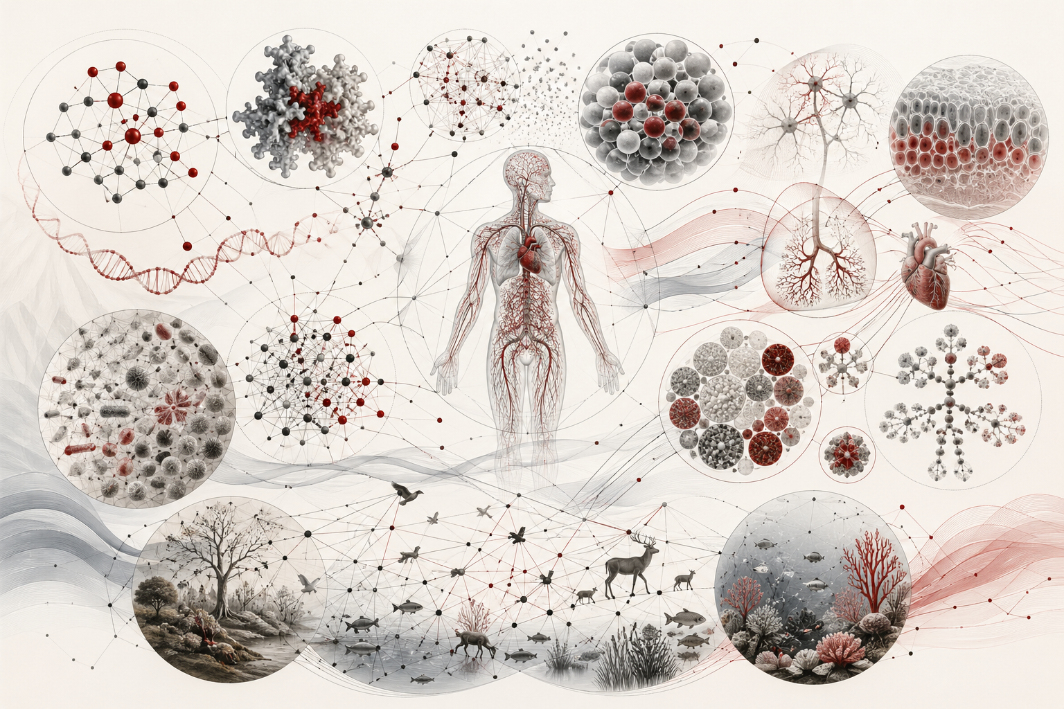
The article is written for biologists, ecologists, marine biologists, systems biologists, computational biologists, biomedical researchers, microbiologists, physiologists, biotechnology scientists, network scientists, engineers, environmental scientists, applied mathematicians, and scientific readers who need a rigorous but usable framework for biological complexity. It treats networks not as decorative diagrams, but as analytical structures for studying function, robustness, vulnerability, adaptation, disease, ecosystem stability, and biological organization across scales.
The article also extends the discussion into reproducible computational practice through graph representation, adjacency matrices, degree distributions, clustering, centrality, modularity, diffusion on networks, gene-regulatory motifs, ecological food-web scaffolds, microbiome association networks, physiological dependency graphs, robustness simulations, sensitivity analysis, R workflows, Python workflows, SQL provenance structures, and a linked full-stack GitHub repository containing Python, R, Julia, Fortran, Rust, Go, C, C++, SQL, notebooks, data files, validation notes, and reproducibility documentation.
Why Networks Matter in Biology
Networks matter in biology because living systems are built from relationships. Genes regulate other genes. Proteins bind, modify, inhibit, activate, transport, and degrade other molecules. Cells signal to neighboring cells. Organs communicate through hormones, nerves, immune signals, blood flow, metabolites, and mechanical forces. Organisms interact through predation, competition, symbiosis, parasitism, mutualism, and ecosystem engineering. Microbes exchange metabolites and alter chemical environments. Species form food webs, pollination networks, host-parasite networks, and nutrient-cycling systems.
A biological network is a structured representation of those relationships. Nodes may represent genes, proteins, cells, neurons, organs, species, microbial taxa, metabolites, individuals, populations, or habitats. Edges may represent regulation, binding, flow, communication, interaction, transmission, dependence, correlation, or causal influence. The network does not replace biological knowledge; it organizes biological knowledge so that patterns of interaction become analyzable.
This matters because biological function often depends less on isolated parts than on how parts are connected. The same protein can behave differently depending on network context. A species can have large ecological influence because of its position in a food web. A mutation can be buffered if redundant pathways exist, or catastrophic if it affects a hub. A physiological system can remain stable because multiple feedback loops compensate for disturbance. A microbial community can resist invasion because its interaction network occupies available ecological niches.
Network biology therefore helps answer questions that reductionist lists cannot answer by themselves. Which components are central? Which modules perform distinct functions? Which interactions stabilize the system? Which nodes create vulnerability? Which pathways compensate after damage? Which connections allow information, energy, disease, or perturbation to spread?
The practical value of a network perspective is that it forces the analyst to specify relationships rather than merely place objects near one another in a diagram. A network can distinguish physical binding from transcriptional regulation, trophic consumption from habitat co-occurrence, anatomical connection from statistical similarity, and material flow from causal influence. Those distinctions determine what questions the model can answer.
In 2026, network biology increasingly operates across data layers that were once analyzed separately. Single-cell atlases, spatial molecular maps, curated pathway databases, perturbation screens, clinical phenotypes, ecological observations, and mechanistic models can now be connected within common analytical systems. This creates scientific opportunity, but it also raises the cost of vague edges, uncertain provenance, and untested causal claims.
From Parts to Relations
Biology has always required attention to parts: cells, tissues, organs, genes, enzymes, species, populations, and ecosystems. But modern biology increasingly recognizes that parts gain meaning through relations. A gene’s function depends on regulatory context. An enzyme’s role depends on pathway structure. A neuron’s importance depends on circuit connectivity. A predator’s influence depends on food-web position. A microorganism’s effect depends on community composition and chemical exchange.
This does not mean parts are unimportant. It means that biological explanation must connect parts to systems. Molecular biology identifies components and mechanisms. Network biology asks how components interact. Systems biology asks how those interactions generate function, regulation, dynamics, adaptation, and failure.
The difference is visible across scales. In genomics, a gene list may tell researchers which genes are differentially expressed, but a regulatory network can suggest which transcription factors coordinate the response. In ecology, a species inventory may tell researchers what is present, but an interaction network can suggest how energy, pollination, disease, or predation flows through the community. In physiology, a hormone value may indicate a state, but a systems model can show how organs, signals, feedback loops, and delays shape that state.
The move from parts to relations is not a rejection of biological detail. It is an expansion of biological explanation.
The relational view also changes intervention. If function is distributed across a network, removing or modifying one component may trigger compensation, rerouting, feedback, or state change elsewhere. A gene knockout may activate a paralog. A drug may shift signaling through an alternative pathway. Removal of a predator may reorganize several trophic levels. A microbial treatment may alter metabolites that affect organisms not directly targeted.
Network analysis is therefore most useful when it is paired with a theory of mechanism. Structure tells researchers what is connected; dynamics tell them how those connections transmit constraint, information, material, or perturbation.
Nodes, Edges, Layers, and Model Boundaries
Every biological network begins with modeling choices. A node may represent a gene, transcript, protein isoform, protein complex, metabolite, reaction, cell state, cell type, species, habitat patch, organ, patient, or clinical phenotype. An edge may represent direct binding, regulatory influence, reaction participation, spatial adjacency, temporal succession, statistical association, trophic interaction, shared disease involvement, or predicted causality. These choices are not interchangeable.
Direction matters when an interaction has an origin and destination. Sign matters when an interaction activates or inhibits. Weight may represent abundance, flux, confidence, effect size, probability, distance, or frequency. Time matters when connections appear, disappear, strengthen, or reverse. Layer matters when the same nodes participate in molecular, spatial, physiological, social, or ecological relations simultaneously.
| Model choice | Biological question | Failure if unspecified |
|---|---|---|
| Node identity | What biological entity is being represented? | Isoforms, cell states, or species may be collapsed incorrectly. |
| Edge meaning | What relationship does a connection assert? | Association may be interpreted as mechanism. |
| Direction and sign | Who influences whom, and how? | Activation and inhibition may be treated as equivalent. |
| Weight and confidence | How strong and how well supported is the relation? | Weak predictions may appear equal to validated interactions. |
| Boundary | What system and context are included? | Important external regulators or affected systems may disappear. |
| Time and layer | When and in which biological domain does the edge exist? | A dynamic multilayer process may be frozen into one static graph. |
A network is therefore not discovered as a finished object. It is constructed from observations, definitions, databases, assumptions, and evidence thresholds. Responsible analysis records those choices as part of the scientific result.
Biological Complexity and Emergence
Biological complexity arises when many interacting components produce system-level behavior that cannot be understood by examining each component in isolation. Emergence does not mean mystery. It means that the behavior of the whole depends on interactions among parts.
A flock moves through local interactions among individuals. A tissue develops through signaling, gradients, mechanics, and gene regulation. An immune response emerges from cells, cytokines, tissues, antigens, memory, and feedback. A microbial community produces chemical dynamics that no single organism produces alone. A forest regulates water, carbon, soil, microclimate, habitat, and biodiversity through coupled ecological processes.
Emergence is central to life because organisms are organized systems. Molecules become pathways. Pathways become cells. Cells become tissues. Tissues become organs. Organs become organisms. Organisms become populations. Populations become communities. Communities become ecosystems. At each level, new properties appear because components interact under constraints.
Biological complexity is therefore not merely “many things at once.” It is structured interdependence across scales. Networks provide one way to make that interdependence visible and computable.
Emergent behavior can often be investigated through controlled simplification. Researchers may identify a minimal circuit that oscillates, a feedback architecture that creates bistability, a food-web configuration that supports persistence, or a spatial interaction pattern that produces tissue organization. The claim is not that the simplified model contains the whole organism or ecosystem. The claim is that a specified interaction structure can generate a specified system-level behavior.
Complexity becomes scientifically useful when the analyst can connect a macro-level pattern to measurable interactions, constraints, and state variables. Emergence should therefore invite deeper mechanism, not become an excuse for vague holism.
Dynamic Networks and Biological State Transitions
Most biological networks are dynamic. Gene regulation changes during development, stress, infection, and differentiation. Protein interactions depend on localization, modification, concentration, and cell state. Physiological coupling changes across sleep, exercise, disease, and treatment. Ecological interactions vary with season, abundance, climate, and disturbance. A static network is often an average over many states.
Dynamic network analysis distinguishes topology from state. Topology describes possible or observed relationships. State describes the current activity, abundance, occupancy, or flux associated with nodes and edges. A network may retain the same topology while changing activity, or it may rewire by gaining and losing edges. Both processes can create biological transitions.
State transitions may be gradual, threshold-driven, stochastic, or history-dependent. Positive feedback can stabilize alternative states. Slow variables can move a system toward a tipping point. Transient perturbations can create long-lasting memory through epigenetic, ecological, immunological, or developmental mechanisms. For this reason, time-resolved measurement and perturbation are often more informative than one cross-sectional network.
A strong dynamic model states the time scale, update rule, initial condition, boundary condition, and observation process. Without those elements, arrows on a pathway diagram do not yet constitute a model of biological behavior.
Genes, Proteins, and Molecular Networks
At the molecular level, biological networks include gene-regulatory networks, protein-protein interaction networks, metabolic networks, signaling networks, RNA regulatory networks, and epigenetic regulatory systems. These networks help explain how molecular components coordinate cellular function.
Gene-regulatory networks show how transcription factors, enhancers, repressors, chromatin states, noncoding RNAs, and signaling pathways shape gene expression. A gene may activate another gene, repress a competitor, participate in a feedback loop, or belong to a broader module controlling development, stress response, metabolism, or cell fate. Such networks are important because cells do not express genes independently. They coordinate expression programs.
Protein networks show physical and functional interactions among proteins. Some proteins are highly connected hubs. Others serve as bridges between modules. Some interactions are stable; others are context-dependent. Protein networks can reveal pathway organization, disease mechanisms, drug targets, and effects of mutation.
Metabolic networks represent biochemical reactions and flows. Nodes may represent metabolites or reactions, and edges may represent transformation or shared substrates. These networks show how cells manage energy, biosynthesis, detoxification, signaling, and material exchange. They are especially important in microbiology, biotechnology, cancer metabolism, systems biology, and metabolic engineering.
The key point is that molecular biology is not only molecular. It is relational, dynamic, and systemic.
Modern molecular networks are increasingly evidence-layered. A direct biochemical interaction may be supported by structural measurement, affinity assays, co-immunoprecipitation, proximity labeling, or perturbation. A regulatory edge may be supported by chromatin accessibility, transcription-factor binding, expression change, reporter assays, and genetic intervention. Database integration should preserve these evidence types rather than flattening them into an undifferentiated edge.
Curated resources such as Reactome organize reactions and pathways with stable identifiers and literature support, while exchange platforms such as NDEx allow networks to be stored, queried, shared, and published in machine-readable formats. These resources make network knowledge more reusable, but they do not eliminate context dependence or incompleteness.
Gene-Regulatory Networks and Causal Inference
Gene-regulatory networks seek to describe how transcription factors, regulatory elements, chromatin states, noncoding RNAs, signaling pathways, and feedback loops shape expression programs. Network inference often begins with covariation, but co-expression alone does not establish direct regulation. Two genes may correlate because they share a regulator, respond to the same environment, reflect changing cell composition, or occupy the same developmental trajectory.
Stronger inference combines multiple evidence types. Chromatin accessibility can identify candidate regulatory regions. Motif analysis can nominate transcription factors. Chromatin conformation can connect distal elements to promoters. Time ordering can constrain possible direction. Perturbation experiments can test whether changing one regulator alters predicted targets. Single-cell multi-omics and spatial data can add cell-state and tissue context.
- Association: two variables move together under the observed sampling process.
- Prediction: one set of measurements helps forecast another in held-out data.
- Mechanistic plausibility: sequence, binding, localization, or pathway knowledge supports the edge.
- Causal evidence: intervention changes the predicted downstream state under defined conditions.
A responsible regulatory network labels which level of support each edge has achieved. The graph should not imply that every inferred connection has been experimentally established.
Metabolic Networks and Constraint-Based Modeling
Metabolic networks represent transformations of matter and energy. Depending on the representation, nodes may be metabolites, reactions, enzymes, genes, or compartments. Edges may indicate substrate-product relationships, enzyme control, transport, or shared participation in a reaction. Unlike many association networks, metabolic networks are constrained by stoichiometry and conservation.
S v = 0
\]
Interpretation: The stoichiometric matrix \(S\) and flux vector \(v\) express a steady-state mass-balance constraint. Each metabolite is produced and consumed according to the encoded reactions.
Flux-balance analysis adds bounds and an objective to identify feasible metabolic states. The method is powerful for microbial physiology, metabolic engineering, cancer metabolism, and community models, but results depend on the reaction set, compartment definitions, exchange bounds, objective assumptions, and environmental conditions.
Metabolic networks also illustrate why topology alone is insufficient. Two reactions can be connected structurally while carrying negligible flux. Alternative pathways may become active only after gene deletion or nutrient change. Isotopic tracing, metabolomics, enzyme measurements, and perturbation improve the biological interpretation of predicted flux.
Cellular Systems and Regulatory Architecture
Cells are organized through regulatory architecture. They sense external conditions, process signals, regulate gene expression, allocate energy, repair damage, divide, differentiate, migrate, communicate, and die. These processes depend on networks of molecules and compartments.
Cellular networks often contain recurring motifs: feedback loops, feedforward loops, toggle switches, oscillators, cascades, checkpoints, and redundancy. These motifs shape timing, stability, noise filtering, memory, sensitivity, and response. For example, negative feedback can stabilize a pathway, positive feedback can create commitment, and feedforward loops can filter transient noise.
Cellular complexity is also spatial. Molecules are not floating in a uniform space. They are organized across membranes, organelles, cytoskeleton, nuclei, vesicles, gradients, microdomains, and tissue contexts. A signaling pathway may behave differently depending on localization. A gene-regulatory network may depend on chromatin architecture. A metabolic network may depend on compartmentalization.
A systems view of the cell therefore requires more than a pathway diagram. It requires understanding how molecular interactions are organized in time, space, concentration, physical structure, feedback, and cellular state.
Cell state is not determined by a single pathway. It emerges from coupled regulation among transcription, translation, metabolism, organelle function, mechanical context, and extracellular signaling. This coupling explains why the same mutation or drug can produce different effects across cell types and microenvironments.
Synthetic and systems biology often use circuit abstractions because motifs reveal design principles. Yet a motif that works in one chassis may fail in another because resource competition, growth rate, burden, noise, and host regulation alter circuit behavior. Network design therefore requires context-aware validation.
Single-Cell, Spatial, and Tissue Network Biology
Single-cell and spatial technologies have shifted network biology from averaged molecular profiles toward heterogeneous, organized tissues. The Human Cell Atlas Data Portal now contains tens of millions of cells across hundreds of projects, while NIH HuBMAP focuses explicitly on the spatial organization, specialization, and interactions of healthy human cells. These initiatives make cell identity and tissue context central to systems analysis.
A tissue network may include cell types or cell states as nodes and ligand-receptor communication, physical adjacency, lineage transition, shared niche, or regulatory influence as edges. Spatial proximity can strengthen a communication hypothesis, but proximity alone does not prove signaling. Ligand and receptor expression may not establish secretion, activation, transport, or downstream response.
Single-cell network inference also faces measurement challenges: sparse counts, sampling imbalance, batch effects, dissociation bias, cell-state continua, donor heterogeneity, and uncertain annotation. Aggregating cells can stabilize estimates but hide rare states. Modeling every cell separately can amplify technical noise. Multilevel designs that preserve donor and tissue structure are often necessary.
Spatial and temporal context is especially important in development, cancer, immunity, repair, and neurobiology. A regulatory edge may exist only in one cell state; a communication path may appear only at an anatomical boundary; and a disease module may depend on a specific microenvironment.
Physiological Networks and Organismal Integration
Organisms are networks of physiological regulation. The nervous system, endocrine system, immune system, cardiovascular system, respiratory system, digestive system, renal system, musculoskeletal system, and microbiome communicate through signals, flows, pressures, metabolites, hormones, neural impulses, immune mediators, and mechanical forces.
Physiology depends on integration. Blood glucose regulation involves pancreas, liver, muscle, adipose tissue, gut hormones, nervous system, metabolism, diet, activity, and circadian rhythms. Blood pressure regulation involves heart, vessels, kidneys, hormones, neural control, fluid balance, and vascular resistance. Immune regulation involves pathogens, tissues, cytokines, barriers, lymphoid organs, microbiome signals, memory cells, and inflammatory control.
This makes organismal biology a network problem. A disease in one organ can affect another. A drug can produce systemic effects through multiple pathways. A stressor can propagate through endocrine, immune, metabolic, and neural systems. Robust health depends on regulatory networks that can absorb disturbance, compensate, and adapt.
Network thinking helps physiology move from isolated variables to systems of interdependence. A single biomarker may matter, but its meaning depends on the network state.
Physiological networks operate across sharply different time scales. Neural signaling may occur in milliseconds, hormonal regulation over minutes or hours, immune remodeling over days, and structural adaptation over months or years. Integrative models must therefore specify which dynamics are resolved and which are treated as slowly varying context.
Clinical measurements also observe only part of the network. A biomarker is a projection of a larger physiological state. Network physiology can help interpret interacting signals, but model complexity should be matched to the evidence and intended decision.
Microbiomes and Community Network Structure
Microbiomes are biological networks of microbial taxa, metabolites, hosts, immune signals, environmental conditions, and ecological interactions. Microbes compete for resources, produce inhibitory compounds, exchange metabolites, form biofilms, communicate through quorum sensing, alter pH and oxygen conditions, and interact with host tissues.
Microbiome complexity illustrates why correlation is not enough. Two taxa may co-occur because they interact directly, because they share an environmental preference, because both respond to a third organism, or because sequencing and sampling artifacts create apparent association. Network analysis can help identify patterns, but biological interpretation requires caution.
Still, microbial network thinking is valuable. It can help identify keystone taxa, metabolic guilds, community modules, dysbiosis patterns, host-microbe interactions, environmental drivers, and potential intervention points. In biotechnology, microbial consortia can be designed or managed by considering cooperation, competition, nutrient exchange, and stability. In ecology, microbial networks help explain decomposition, nutrient cycling, soil fertility, ocean productivity, and biogeochemical transformation.
The microbiome shows that biological complexity is often distributed. No single organism “contains” the system. Function emerges from community interaction.
Microbiome association networks are particularly vulnerable to compositional effects because sequencing data usually record relative rather than absolute abundance. An apparent negative edge can arise when one taxon expands and forces the proportions of others downward. Shared environmental drivers and unmeasured metabolites can also create indirect associations.
Stronger microbial network studies incorporate absolute abundance where possible, environmental covariates, time series, metabolite measurements, culture or synthetic-community experiments, and perturbations such as diet, antibiotics, phage, or nutrient change. Network edges should be treated as hypotheses to test, not automatically as ecological interactions.
Ecological Networks and the Interdependence of Life
Ecology is fundamentally networked. Species interact through predation, herbivory, competition, mutualism, parasitism, commensalism, decomposition, facilitation, and habitat engineering. Ecosystems also include abiotic flows of water, nutrients, carbon, energy, temperature, disturbance, and material transport.
Food webs represent trophic relationships. Pollination networks represent plant-pollinator interactions. Host-parasite networks represent disease and dependency. Seed-dispersal networks represent movement and reproduction. Habitat networks represent landscape connectivity. Biogeochemical networks represent flows among organisms, soils, water, atmosphere, and sediments.
Ecological networks matter because ecosystem stability often depends on interaction structure. Redundancy may buffer loss. Highly connected species may stabilize or destabilize the system depending on context. Modular structure may contain disturbance. Weak interactions may dampen oscillations. Loss of a keystone species may trigger cascading effects. Habitat fragmentation may break dispersal networks. Climate stress may rewire interactions.
Ecological complexity therefore cannot be understood only through species counts. Biodiversity includes composition, function, interaction, evolutionary history, and network structure. The protection of life requires understanding how life is connected.
Ecological networks are often multilayered. The same species may participate in trophic, mutualistic, competitive, parasitic, and habitat-forming interactions. A plant can be eaten by herbivores, pollinated by insects, dispersed by birds, infected by pathogens, and connected indirectly through soil organisms. Treating these layers separately can clarify mechanism; integrating them can reveal cross-layer dependencies.
Sampling incompleteness is a central uncertainty. Rare interactions are difficult to observe, interaction frequency changes with abundance, and networks may differ across seasons or habitats. Comparing networks therefore requires attention to sampling effort, detection, taxonomic resolution, spatial grain, and temporal coverage.
Multilayer, Temporal, and Spatial Networks
Many biological systems require more than one adjacency matrix. A multilayer network represents different relationship types, scales, or contexts while retaining links among layers. Layers may correspond to molecular modalities, tissues, time points, habitats, interaction types, species, patients, or experimental conditions.
Temporal networks record when interactions occur. Spatial networks record where nodes and edges are located. Multiplex networks allow the same nodes to participate in several edge types. Interdependent networks connect distinct systems, such as metabolism and gene regulation, host physiology and microbiome function, or habitats and species movement.
\mathcal{G}=\{G^{[1]},G^{[2]},\ldots,G^{[L]}\}
\]
Interpretation: A multilayer system contains layer-specific graphs \(G^{[\ell]}\). Cross-layer links encode correspondence or interaction among nodes represented in different layers.
The analytical advantage is biological fidelity. The disadvantage is increased parameterization, missingness, alignment difficulty, and interpretive complexity. Layer integration should be justified by the question rather than performed merely because multiple datasets are available.
Modularity, Hierarchy, and Biological Organization
Biological systems are often modular. A module is a cluster of components that interact more strongly with one another than with the rest of the system. Modules can appear in gene regulation, metabolism, protein interaction, neural circuits, organs, developmental programs, microbial communities, and ecosystems.
Modularity supports biological complexity because it allows systems to combine specialization with integration. A metabolic module can perform a pathway function. A gene module can coordinate development. An organ can specialize while communicating with the rest of the body. An ecological guild can perform a shared role. Modules can also evolve, adapt, fail, or be modified without requiring the whole system to change at once.
Biological systems are also hierarchical. Molecules form pathways, pathways form cells, cells form tissues, tissues form organs, organs form organisms, organisms form populations, and populations form ecosystems. But hierarchy is not always strictly top-down. Lower levels constrain higher levels, while higher-level contexts feed back onto lower levels. Tissue environments regulate cells. Ecosystems shape evolutionary pressure. Organismal behavior changes ecological networks.
Modularity and hierarchy help explain how biology can be both robust and flexible. Systems can maintain local organization while adapting globally. But modularity can also hide failure, create bottlenecks, or compartmentalize dysfunction until thresholds are crossed.
Modules are not unique facts waiting to be read from a graph. Community-detection algorithms optimize different criteria and can return different partitions. Results may change with resolution parameters, edge weights, negative edges, or stochastic initialization. Biological modules should therefore be evaluated for stability, functional coherence, spatial or temporal context, and response to perturbation.
Hierarchical organization may also be overlapping rather than nested. A protein can participate in several complexes, a cell can transition among states, and a species can connect multiple ecological guilds. Overlap and context are often biologically meaningful rather than methodological inconveniences.
Network Motifs, Feedback, and Biological Control
Network motifs are recurring local interaction patterns that can implement recognizable dynamic functions. Negative autoregulation can accelerate response and reduce variability. Positive feedback can produce persistence or bistability. Coherent feedforward loops can filter short inputs. Incoherent feedforward loops can generate pulses or adaptation. Coupled feedback can produce oscillations.
Motif interpretation requires more than counting topology. Interaction sign, strength, delay, saturation, degradation, and noise determine behavior. The same three-node pattern can behave differently under different kinetics. A motif may also appear frequently because of degree structure or data-generation bias rather than selection for a function.
\frac{dx}{dt}=f(x,u,\theta)
\]
Interpretation: The state vector \(x\) changes under inputs \(u\) and parameters \( heta\). Network topology constrains the possible interactions, while the functions and parameters determine the actual dynamics.
Control questions ask whether a system can be moved from one state to another, which inputs are required, and which measurements are sufficient to infer state. In biology, mathematical controllability is only a starting point. Feasible intervention also depends on delivery, toxicity, timing, adaptation, and ethical constraints.
Robustness, Fragility, and Network Failure
Robustness is the ability of a biological system to maintain function despite perturbation. Biological networks can be robust because of redundancy, feedback, modularity, distributed control, alternative pathways, repair mechanisms, and adaptive response. Cells survive mutations because pathways compensate. Organisms maintain homeostasis because physiological systems regulate. Ecosystems recover from disturbance when species and processes overlap functionally.
But robustness can coexist with fragility. A network may tolerate random loss but fail after targeted removal of hubs. A physiological system may compensate for years before abrupt disease. A microbial community may resist disturbance until a tipping point. An ecosystem may appear stable until a keystone interaction is disrupted. A metabolic network may reroute flux until one bottleneck collapses function.
This makes network structure essential for understanding risk. Vulnerability depends not only on how many parts exist, but on how they are connected. A highly connected node may be essential. A bridge between modules may be critical. A redundant pathway may reduce risk. A tightly coupled system may propagate failure rapidly.
Network failure is therefore a biological and systems problem. It includes disease, ecosystem collapse, developmental disruption, immune dysregulation, metabolic breakdown, population extinction, and engineered biological instability.
Robustness should be defined relative to a function and perturbation. Retaining a giant connected component is not the same as retaining respiration, immune tolerance, developmental patterning, pollination, or metabolic output. Structural and functional robustness can diverge.
Biological networks can also be robust yet evolvable. Redundancy and modularity buffer some changes while permitting variation in others. The same architecture that protects normal function may protect a disease network or invasive ecosystem state from intervention.
Perturbation Propagation and Tipping Points
Perturbations propagate through biological networks according to topology, dynamics, state, and feedback. A molecular perturbation can change expression, metabolism, and cell behavior. A physiological perturbation can recruit compensatory organs and signals. An ecological disturbance can spread through trophic and spatial connections. Propagation is rarely uniform.
Small perturbations may decay, be amplified, or redirect the system into another basin of attraction. Repeated weak stress can erode resilience even when each event appears recoverable. Delays can hide accumulating risk. Near a critical transition, recovery may slow and variance may increase, although such indicators are not universal.
Network propagation models can prioritize downstream nodes or candidate disease modules, but their results depend on edge direction, normalization, diffusion parameters, and the starting signal. Validation should compare predicted propagation with time-resolved measurements or perturbation experiments.
Tipping-point language should be used carefully. A sharp model transition does not prove that a real organism or ecosystem has a precisely known threshold. It identifies conditions under which nonlinear change is plausible and worth monitoring.
Evolution, Adaptation, and Network Rewiring
Biological networks evolve. Gene duplication can create redundancy and new regulation. Mutations can alter binding, expression, interaction specificity, or network topology. Developmental systems can change through regulatory rewiring. Microbial communities adapt through mutation, migration, horizontal transfer, and ecological sorting. Ecological networks reorganize as distributions, abundances, and behaviors change.
Selection acts on phenotypes generated by networks rather than on isolated components alone. Network architecture can channel variation, buffer mutations, and create trade-offs. Modularity may permit local adaptation; pleiotropy may constrain change; feedback may stabilize states; and environmental variation may favor flexible responses.
Comparative network analysis can identify conserved modules and lineage-specific rewiring, but comparison requires harmonized node identities, orthology, evidence standards, and sampling. Missing data can mimic evolutionary loss. Differences in experimental technology can mimic biological divergence.
Adaptation also matters during intervention. Pathogens evolve resistance, tumors rewire signaling, ecosystems shift species interactions, and engineered circuits mutate. Network models should therefore include plausible adaptive responses when decisions extend beyond short experimental windows.
Disease as Network Dysregulation
Many diseases can be understood as network dysregulation. Cancer involves gene-regulatory changes, signaling rewiring, metabolism, immune evasion, tissue interactions, vascularization, and evolutionary dynamics. Diabetes involves endocrine, metabolic, inflammatory, behavioral, genetic, and physiological networks. Autoimmune disease involves immune recognition, tolerance, inflammation, tissue feedback, and genetic susceptibility. Neurodegenerative disease involves protein networks, cellular stress, metabolism, inflammation, synaptic networks, and repair systems.
A network view does not reduce disease to a diagram. It expands disease explanation beyond a single cause. It asks how pathways interact, how perturbations spread, how compensatory mechanisms fail, how modules rewire, and how intervention at one point affects the broader system.
This is especially important for complex diseases. A drug may target one pathway but trigger compensation through another. A biomarker may indicate one network state but not the whole disease process. A genetic variant may matter only in a particular regulatory context. A therapy may work for one network subtype and fail for another.
Network medicine, systems pharmacology, and computational biology all emerge from this recognition: disease often lives in the pattern of relationships, not merely in isolated parts.
Disease networks are heterogeneous across people, tissues, and time. A diagnostic label may contain several molecular or physiological states. Conversely, different diagnoses may share pathways or comorbid network modules. Network medicine seeks to connect these patterns without assuming that one graph fits every patient.
The translational challenge is validation. A disease module should predict something beyond the data used to build it: response to perturbation, clinical outcome, therapeutic sensitivity, or reproducible localization in independent evidence.
Network Medicine and Disease Modules
Network medicine represents disease genes, proteins, pathways, phenotypes, exposures, and drugs within structured biological networks. A disease module is a subnetwork whose components are more closely connected to one another or to a disease process than expected under an appropriate null model. The approach can connect dispersed genetic findings to shared mechanisms.
Module discovery can use seed expansion, random walks, diffusion, community detection, graph neural methods, or integration of multiple evidence types. Each method introduces assumptions about the interactome, edge confidence, missing nodes, degree bias, and disease labels. Highly studied proteins may appear central partly because they have more recorded interactions.
Useful disease modules should be evaluated for reproducibility, functional coherence, specificity, external validation, and sensitivity to the background network. They may support target discovery, biomarker interpretation, patient stratification, comorbidity analysis, and drug repurposing, but they are not clinical conclusions by themselves.
Current network medicine increasingly integrates genomics, transcriptomics, proteomics, metabolomics, spatial data, and clinical information. The scientific opportunity is to connect mechanisms across layers; the main risk is to produce a large integrated graph whose apparent comprehensiveness exceeds its evidential reliability.
Systems Pharmacology and Polypharmacology
Drugs rarely act on only one biological component. Intended targets, off-targets, metabolites, transporters, physiological feedback, and disease-state differences shape response. Systems pharmacology represents these relationships across drug-target, pathway, tissue, phenotype, and adverse-event networks.
Polypharmacology can be harmful when off-target activity creates toxicity, but it can also be beneficial when coordinated modulation of several targets is required. Combination therapy can block compensatory pathways or address heterogeneous disease states. Network models can nominate combinations, but interaction risk, dose, timing, exposure, and clinical context must be evaluated experimentally.
Drug repurposing methods often use network proximity between drug targets and disease modules. Results depend strongly on interactome completeness, target annotation, degree structure, and disease-gene selection. A high-ranked candidate is a hypothesis for pharmacological testing, not evidence of efficacy.
Mechanistic pharmacology can combine network structure with pharmacokinetics, pharmacodynamics, cell-state models, and patient heterogeneity. Such integration is promising, but uncertainty should remain visible rather than disappearing into one score.
Artificial Intelligence, Mechanistic Modeling, and Digital Twins
Machine learning can discover representations, predict interactions, classify states, and prioritize perturbations in large biological datasets. Mechanistic models encode explicit biological relationships, conservation laws, kinetics, and feedback. The strongest systems workflows increasingly combine these approaches rather than treating them as alternatives.
AI can help estimate missing parameters, emulate expensive simulations, infer latent states, or identify candidate network structures. Mechanistic constraints can improve plausibility and extrapolation. Yet hybrid models still inherit bias from training data, uncertain annotations, batch effects, and incomplete mechanisms. Interpretability claims should specify whether the model exposes correlations, causal hypotheses, or governing equations.
Biological digital twins aim to maintain a computational representation of an organism, organ, cell system, bioprocess, or ecosystem that updates with data and supports simulation. This is an aspirational continuum rather than one standardized technology. A digital twin requires defined state variables, observation models, validation criteria, update rules, uncertainty, and a decision boundary.
For clinical or ecological use, high apparent accuracy is insufficient. Models need external validation, calibration, monitoring for drift, documented failure modes, and human oversight. AI should accelerate hypothesis generation and model comparison without hiding uncertainty or replacing experimental accountability.
Multi-Omics Integration and Cross-Scale Modeling
Multi-omics integration combines molecular layers such as genome, epigenome, transcriptome, proteome, metabolome, and microbiome. The objective is not simply to place all measurements in one matrix. It is to identify relationships that help explain state, mechanism, variation, or response across layers.
Integration can occur through shared latent spaces, linked factor models, pathway aggregation, multilayer graphs, Bayesian models, or mechanistic constraints. Each choice determines which signals are aligned and which differences are preserved. Overaggressive alignment can erase real biological variation. Weak alignment can leave modalities disconnected.
Cross-scale modeling is harder because molecular, cellular, tissue, organismal, and ecological models operate with different entities and time scales. Bridging variables must be biologically justified. For example, gene expression may influence protein activity, but translation, degradation, modification, localization, and feedback intervene. Cellular states may influence tissue function, but spatial organization and mechanics matter.
Integration should therefore be evaluated by whether it improves a defined task, predicts independent measurements, or supports a testable mechanistic explanation. More layers do not automatically produce more knowledge.
Network Inference from Observational Data
Many biological networks are inferred because direct measurement of every interaction is impossible. Correlation, partial correlation, mutual information, graphical models, regression, time-lag methods, and machine learning can identify candidate relationships. Inference quality depends on sample size, noise, heterogeneity, experimental design, and the relationship between measured variables and biological entities.
High-dimensional inference is underdetermined: many networks can explain the same observations. Sparsity assumptions, priors, pathway constraints, and regularization reduce the solution space but also shape the result. Cross-validation can test prediction but may not establish causal structure. Stability selection and bootstrap analysis can show whether edges persist under resampling.
- Confounding: an unmeasured variable influences both nodes.
- Compositionality: relative measurements induce dependencies.
- Batch effects: technical structure creates apparent modules.
- Cell mixture: changing composition mimics regulation.
- Selection bias: sampled units do not represent the target system.
- Temporal ambiguity: cross-sectional data cannot establish ordering.
The output of observational inference should usually be a ranked, uncertainty-aware network hypothesis. Its value lies in organizing follow-up experiments, not in eliminating the need for them.
Causality, Perturbation, and Experimental Validation
Causal network claims require evidence about interventions or defensible causal assumptions. Genetic knockouts, CRISPR interference or activation, pharmacological perturbation, optogenetics, environmental manipulation, species removal, controlled community assembly, and natural experiments can reveal how changing one component affects others.
Perturbation design must consider dose, timing, adaptation, off-target effects, compensation, and measurement coverage. A perturbation can affect several nodes directly. A null response may reflect inadequate delivery rather than absence of an edge. A downstream change may be indirect. Controls and orthogonal validation remain essential.
Causal discovery methods can combine conditional independence, temporal ordering, instrumental variables, invariance across environments, or structural models. These methods are useful when assumptions are explicit and partially testable. They should not be presented as automated causal truth from observational omics.
A mature network program cycles between inference and intervention: construct a network, identify discriminating predictions, perturb the system, compare outcomes with predictions, revise the network, and record what changed.
Uncertainty, Identifiability, and Model Ensembles
Network models contain several forms of uncertainty. Structural uncertainty concerns which nodes and edges belong. Parametric uncertainty concerns weights, rates, and thresholds. State uncertainty concerns the current biological condition. Observation uncertainty concerns how data were generated. Scenario uncertainty concerns future environments or interventions.
Identifiability asks whether available data can distinguish parameter values or network structures. A model may fit perfectly while several alternative explanations remain possible. More complex models often increase this problem. Profile likelihood, posterior distributions, sensitivity analysis, perturbation design, and model comparison can reveal what is and is not identifiable.
Model ensembles retain several plausible networks or parameter sets rather than selecting one prematurely. Predictions that remain stable across the ensemble are more robust to uncertainty. Predictions that vary reveal where new measurements would be most valuable.
Uncertainty should travel into downstream rankings. Hub status, module membership, disease proximity, robustness, and intervention priority can all change when uncertain edges are resampled. Reporting only the final graph creates false precision.
Network Data Standards, Provenance, and Reproducibility
Network results are difficult to reuse when they exist only as figures. Reproducible network biology stores machine-readable nodes, edges, attributes, evidence, identifiers, licenses, versions, and analysis parameters. Stable identifiers help connect genes, proteins, pathways, species, chemicals, and diseases across resources.
NDEx provides an open platform for storing, sharing, querying, and publishing biological networks, and its documentation recommends the CX2 exchange format for new applications. Cytoscape and related tools support analysis and visualization, while curated pathway resources such as Reactome provide versioned biological knowledge. These infrastructures support reproducibility only when provenance is retained.
- source dataset and access date;
- node and edge definitions;
- identifier namespace and mapping procedure;
- evidence type and confidence;
- filtering and threshold decisions;
- software, package, and database versions;
- random seeds and algorithm parameters;
- layout as presentation metadata rather than biological evidence;
- license and permitted reuse;
- validation results and known limitations.
A published network should be inspectable as data, not merely persuasive as an image.
Mathematical Lens: Network Structure, Dynamics, and Uncertainty
Network mathematics helps separate structural description, dynamic behavior, uncertainty, and intervention. No metric is universally biological. A metric becomes meaningful only after node, edge, boundary, and evidence definitions are established.
Graph and multilayer representation
G=(V,E,W), \qquad \mathcal{G}=\{G^{[1]},\ldots,G^{[L]}\}
\]
Interpretation: A weighted graph contains nodes, edges, and weights. A multilayer system contains several related graphs representing modalities, contexts, or interaction types.
Directed signed adjacency
A_{ij} \in \mathbb{R}
\]
Interpretation: The sign can distinguish activation from inhibition and the magnitude can represent strength or confidence. Zero means no encoded edge, not necessarily biological absence.
Degree and strength
k_i=\sum_j \mathbf{1}(A_{ij}\neq0), \qquad s_i=\sum_j |A_{ij}|
\]
Interpretation: Degree counts encoded connections, while strength aggregates their weights. Both are sensitive to measurement and database coverage.
Local clustering
C_i=\frac{2e_i}{k_i(k_i-1)}
\]
Interpretation: Clustering measures connectivity among neighbors. High values can indicate complexes, local modules, or sampling density.
Modularity
Q=\frac{1}{2m}\sum_{ij}\left(A_{ij}-\gamma\frac{k_i k_j}{2m}\right)\delta(c_i,c_j)
\]
Interpretation: The resolution parameter \(\gamma\) changes the scale at which modules are detected. Module assignments should be checked for stability and biological coherence.
Network dynamics
\frac{dx_i}{dt}=f_i(x_i,u_i)+\sum_j A_{ji}g_{ji}(x_j,x_i)
\]
Interpretation: Node state changes through internal dynamics, inputs, and incoming interactions. Topology constrains the model but does not determine kinetics.
Graph diffusion
x_{t+1}=(1-\lambda)x_t+\alpha P x_t
\]
Interpretation: A normalized propagation matrix \(P\) spreads state or evidence while \(\lambda\) represents loss. Results depend on normalization, seeds, and propagation parameters.
Structural robustness
R(q)=\frac{|C_{\max}(G\setminus S_q)|}{|V|-|S_q|}
\]
Interpretation: After removing a set \(S_q\), robustness is approximated by the fraction of remaining nodes in the largest connected component. Functional robustness may differ.
Edge uncertainty
Z_{ij}^{(b)} \sim \operatorname{Bernoulli}(p_{ij})
\]
Interpretation: In ensemble trial \(b\), an uncertain edge is retained according to support probability \(p_{ij}\). The resulting distribution shows how conclusions depend on edge uncertainty.
Sensitivity of an output
S_{\theta}=\frac{\partial y}{\partial \theta}
\]
Interpretation: Sensitivity measures how a network output changes with a parameter or assumption. Large sensitivity identifies influential uncertainty and possible experimental priorities.
Centrality, modularity, robustness, and diffusion should be reported with the network definition, null model, algorithm, parameters, and uncertainty analysis. A mathematically precise metric can still answer the wrong biological question.
R and Python Workflows
The compact article-level workflows below use small synthetic networks to demonstrate topology, diffusion, and uncertainty. The companion bundle provides a larger standard-library Python implementation, base R diagnostics, synthetic data, tests, generated outputs, and a metric contract.
Python example: topology, clustering, and targeted removal
from collections import defaultdict, deque

edges = [
    ("TF_A", "GENE_B", 0.92),
    ("TF_A", "GENE_C", 0.84),
    ("GENE_B", "PROTEIN_D", 0.76),
    ("GENE_C", "PROTEIN_D", 0.81),
    ("PROTEIN_D", "METABOLITE_E", 0.88),
]

adjacency = defaultdict(set)
for source, target, confidence in edges:
    adjacency[source].add(target)
    adjacency[target].add(source)

degree = {node: len(neighbors) for node, neighbors in adjacency.items()}
ranked = sorted(degree.items(), key=lambda item: (-item[1], item[0]))
print(ranked)

# Targeted-removal diagnostic.
removed = ranked[0][0]
remaining = {node for node in adjacency if node != removed}
start = next(iter(remaining))
seen = {start}
queue = deque([start])
while queue:
    node = queue.popleft()
    for neighbor in adjacency[node]:
        if neighbor in remaining and neighbor not in seen:
            seen.add(neighbor)
            queue.append(neighbor)
print("removed:", removed, "largest_reached_fraction:", len(seen) / len(remaining))
Python example: confidence-aware edge ensemble
import random
from collections import Counter

rng = random.Random(20260804)
edges = [
    ("A", "B", 0.95),
    ("A", "C", 0.80),
    ("B", "D", 0.70),
    ("C", "D", 0.65),
    ("D", "E", 0.90),
]

top_hubs = Counter()
for trial in range(1000):
    degree = Counter()
    for source, target, confidence in edges:
        if rng.random() <= confidence:
            degree[source] += 1
            degree[target] += 1
    if degree:
        hub = sorted(degree, key=lambda node: (-degree[node], node))[0]
        top_hubs[hub] += 1
print(top_hubs)
R example: degree and module summary
edges <- data.frame(
  source = c("A", "A", "B", "C", "D", "E"),
  target = c("B", "C", "D", "D", "E", "F"),
  source_module = c("reg", "reg", "reg", "reg", "met", "met"),
  target_module = c("reg", "reg", "met", "met", "met", "signal")
)

nodes <- sort(unique(c(edges$source, edges$target)))
degree <- sapply(nodes, function(node) {
  sum(edges$source == node | edges$target == node)
})

print(data.frame(node = nodes, degree = degree))
print(with(edges, table(source_module, target_module)))
The synthetic examples deliberately keep the graph small enough to inspect. Real workflows should add identifier validation, evidence provenance, replicate-aware data processing, alternative network definitions, null models, and experimental validation.
GitHub Repository
The article body keeps code compact so the biological argument remains readable. The full bundle expands the examples into topology, module, propagation, targeted-removal, random-removal, and edge-uncertainty workflows using transparent synthetic data.
The continuing repository for this article includes selected examples, expanded workflows, reproducible data structures, provenance documentation, validation notes, and full-stack scientific-computing scaffolding.
Worked Diagnostic: A Multiscale Inflammatory Network
Consider a synthetic research program studying persistent inflammatory disease. The network contains regulatory genes, signaling proteins, immune-cell states, tissue signals, microbial metabolites, and clinical measurements. Edges are labeled by layer, direction, sign, confidence, and evidence type. The goal is not to identify one universal master node. It is to determine which conclusions are robust, which mechanisms remain ambiguous, and which perturbations can discriminate among competing explanations.
Step 1: Define the biological question and boundary
The program asks why a subset of patients remains in a high-inflammatory state after the initiating trigger has resolved. The model includes immune and tissue signaling, selected microbial metabolites, and measured clinical states. It does not claim to represent the complete patient. This boundary prevents the network from being misread as a total model of disease.
Step 2: Build an evidence-layered network
Curated pathway edges, patient-derived associations, spatial cell-neighborhood evidence, and perturbation results are stored separately. Directly validated regulatory edges receive higher support than co-expression edges. Negative and positive regulation are distinguished. The resulting network can be filtered by evidence rather than presenting every edge as equally established.
Step 3: Inspect topology and modules
Degree and weighted-degree summaries identify several connected signaling nodes, but module analysis reveals that one apparent hub is central only because it links two densely measured assay panels. A smaller tissue-feedback node connects immune, epithelial, and metabolic layers. This bridge is less highly connected but more relevant to the persistence hypothesis.
Step 4: Compare states and differential edges
Networks are estimated separately for resolving and persistent inflammation using harmonized sampling. Most edges are shared, but persistent disease shows stronger epithelial-to-immune feedback and weaker regulatory recovery. The analysis checks whether these differences remain after accounting for cell composition, batch, medication, and donor structure.
Step 5: Simulate perturbation and propagation
Diffusion and signed dynamic models compare inhibition of the high-degree signaling hub with interruption of the tissue-feedback bridge. Hub inhibition produces a large immediate change but activates an alternative pathway. Bridge interruption produces a smaller immediate effect but reduces the self-reinforcing loop in more model variants.
Step 6: Test targeted and random failure
Random node removal leaves the network largely connected. Targeted removal of the bridge separates the immune and tissue modules, while removal of the highest-degree node does not. This result is interpreted as structural vulnerability, not proof that the bridge is a safe or effective therapeutic target.
Step 7: Run an uncertainty ensemble
Low-confidence edges are resampled across 2,000 network realizations. The high-degree hub remains highly ranked, but predicted therapeutic benefit varies widely because compensation is uncertain. The tissue-feedback bridge is less prominent in some realizations but retains its role in most models that reproduce persistence. The ensemble therefore separates topological certainty from intervention certainty.
Step 8: Translate the model into experiments
The program chooses experiments that discriminate among the competing models: time-resolved perturbation of the bridge, measurement of the alternative pathway, spatial confirmation of the predicted cell interaction, and replication in an independent cohort. The network is treated as a learning instrument whose value is measured by the quality of the next experiment.
| Finding | Responsible interpretation | Next action |
|---|---|---|
| High-degree signaling hub | Well connected, but may reflect measurement density and compensation. | Test pathway substitution after perturbation. |
| Cross-layer tissue bridge | Potential structural connector; not yet a validated causal target. | Perturb in a context-preserving model and measure both modules. |
| Differential inflammatory edge | State-associated after adjustment; direction still uncertain. | Use time ordering and intervention to test causality. |
| Unstable intervention ranking | Conclusion depends on uncertain edges and parameters. | Collect evidence that reduces the influential uncertainty. |
The worked diagnostic shows why a network study should end with discriminating evidence, not merely a visually compelling graph. The most connected node, the most stable module, and the best intervention target can be different biological objects.
A Practical Method for Network and Systems Biology
A disciplined network study moves from biological question to explicit representation, uncertainty-aware analysis, perturbation, and revision. The following method can be adapted across molecular, cellular, physiological, microbial, ecological, and translational systems.
1. Define the biological question
State what the network must help explain, predict, compare, or decide. Avoid building a graph before defining the intended inference.
2. Set the system boundary
Specify organisms, tissues, cell states, molecular layers, habitats, time scales, and external drivers included or excluded. Record why the boundary is appropriate.
3. Define nodes and edges
State what each entity and relationship means. Distinguish direction, sign, weight, confidence, evidence type, and context.
4. Audit identifiers and provenance
Harmonize identifiers without erasing isoforms, states, taxa, or compartments. Preserve source, version, license, transformation, and access date.
5. Describe the observation process
Document sampling, measurement, detection, normalization, batch structure, missingness, and technical uncertainty that shape the observed network.
6. Build competing network hypotheses
Retain plausible alternative structures or mechanisms. Use priors and constraints transparently rather than hiding them in one final graph.
7. Analyze structure at appropriate scales
Examine connectivity, modules, bridges, motifs, layers, space, and time. Test sensitivity to algorithm and resolution choices.
8. Add dynamics and biological function
Connect structure to state, flow, kinetics, feedback, perturbation, or ecological function. Do not treat topology as a complete explanation.
9. Quantify uncertainty and identifiability
Resample data and uncertain edges, compare models, inspect parameter sensitivity, and report conclusions that are unstable or not identifiable.
10. Validate with perturbation and independent evidence
Use intervention, time-resolved measurement, orthogonal assays, field replication, or independent datasets to test predictions.
11. Translate findings cautiously
Separate descriptive centrality, causal influence, functional necessity, and intervention suitability. Include feasibility, safety, equity, and ecological context where decisions are consequential.
12. Publish the network as a reproducible object
Release machine-readable data, metadata, code, parameters, validation results, uncertainty, and limitations so the network can be audited and improved.
This method treats a biological network as an explicit, revisable scientific model. Its purpose is not to replace experiments or field knowledge, but to make relational hypotheses testable.
Common Pitfalls in Network and Systems Biology
Network analysis can create an impression of depth even when the underlying biological claim is weak. These pitfalls should be checked before interpretation.
- Treating association as causation: Co-expression, co-occurrence, or statistical dependence does not establish direct biological influence.
- Leaving edges undefined: A line can represent binding, regulation, flow, similarity, or confidence; the difference is scientific, not cosmetic.
- Ignoring measurement density: Well-studied genes, proteins, species, or diseases may appear central because they have more recorded edges.
- Flattening context: Interactions can depend on cell state, tissue, environment, developmental stage, season, or treatment.
- Confusing topology with function: Connectivity does not prove necessity, control, or therapeutic suitability.
- Overinterpreting modules: Community partitions depend on algorithms, resolution, and missing edges.
- Ignoring direction, sign, and delay: Unsigned static networks can reverse or erase biological meaning.
- Using one network definition: Thresholds, databases, and identifier mappings can materially change conclusions.
- Forgetting compositional and batch effects: Technical structure can create apparent microbial or omics interactions.
- Hiding uncertainty: A single graph conceals edge, parameter, state, and model uncertainty.
- Validating on the construction data: A network that reproduces its inputs has not necessarily predicted independent biology.
- Publishing only an image: Without machine-readable data, provenance, and code, the result cannot be adequately audited or reused.
The central safeguard is alignment: the biological question, network definition, data-generation process, mathematical method, validation, and claimed conclusion must describe the same system.
Limits, Validation, and Responsible Modeling
Network models can clarify biological complexity, but they can also mislead. A network diagram may look authoritative while hiding uncertainty. An inferred edge may represent correlation rather than direct interaction. A missing edge may reflect incomplete data rather than biological absence. A central node may be important in the model but not in the organism. A module may be mathematically detected but biologically weak. A network may change across time, environment, developmental stage, disease state, or measurement method.
Responsible network biology requires clear definitions. What is a node? What is an edge? Is the edge directed or undirected? Weighted or unweighted? Empirical or inferred? Static or dynamic? Does it represent physical interaction, statistical association, causal regulation, functional similarity, ecological dependence, or material flow? What data support the edge? What uncertainty surrounds it?
Validation is essential. Network results should be compared with experimental evidence, perturbation studies, known biology, independent datasets, mechanistic models, and domain expertise. Robustness analysis should not be reduced to graph metrics alone; biological function matters. A network may remain connected but lose essential function. Another may fragment structurally while preserving local function.
The ethical stakes can be high in medicine, ecology, biotechnology, public health, and conservation. Network models can inform drug targets, disease classification, ecosystem intervention, microbiome manipulation, and engineered biological systems. Such models should be transparent, reproducible, empirically grounded, and communicated with appropriate uncertainty.
Validation should be matched to claim type. A structural claim may be checked against independent interaction evidence. A predictive claim requires held-out or external data. A dynamic claim requires time-resolved behavior. A causal claim requires intervention or defensible assumptions. A translational claim requires performance in the target setting and evaluation of consequences.
Network models can influence clinical, ecological, and biotechnology decisions, so governance matters. Sensitive human data, Indigenous ecological knowledge, proprietary databases, and dual-use biological information may require access controls, community authority, or careful release. Open science does not mean context-free disclosure of every network.
Responsible modeling combines transparency with proportionate safeguards. It makes assumptions visible, avoids claims beyond evidence, and records where human judgment enters the workflow.
Why Network and Systems Thinking Matters
Network and systems thinking matters because many biological problems are problems of interdependence. Disease spreads through networks. Genes regulate one another through networks. Cells coordinate through signaling networks. Physiology depends on organ-system integration. Microbial communities produce functions that no single organism produces alone. Ecosystems depend on interaction networks. Conservation depends not only on species survival, but on the relationships that sustain living systems.
It also matters because biological intervention has consequences beyond the target. A drug may affect multiple pathways. Removing a species may alter a food web. Engineering a microbe may change community dynamics. Modifying a gene may affect developmental networks. Treating one physiological variable may produce compensatory responses elsewhere.
Finally, network and systems thinking helps biology remain scientifically humble. Living systems are complex not because they are unknowable, but because their behavior emerges from organized relationships across scale. Understanding those relationships requires measurement, modeling, experimentation, computation, and interpretation working together.
The 2026 research landscape makes this especially clear. Human cell atlases, spatial molecular maps, pathway databases, network exchanges, and multi-omics programs are creating increasingly rich relational resources. Their scientific value depends on the ability to connect scale without collapsing context, integrate evidence without flattening uncertainty, and translate models into experiments rather than treating integration itself as discovery.
Network thinking is therefore not a claim that everything is connected to everything else. It is a discipline for specifying which relationships matter, how they were measured, what behavior they generate, and what evidence could prove the model wrong.
Conclusion
Networks, systems, and biological complexity provide one of the deepest frameworks for understanding life. Living systems are not merely collections of parts. They are organized patterns of interaction: molecular, cellular, physiological, ecological, evolutionary, and environmental. Their behavior emerges from connections, feedbacks, modules, constraints, flows, and histories.
Network thinking helps biology identify hubs, modules, bridges, vulnerabilities, redundancies, pathways, interaction patterns, and emergent properties. Systems thinking helps connect those structures to function, dynamics, regulation, robustness, disease, resilience, and transformation.
To understand biological complexity is to understand that life is relational. Genes, cells, organisms, species, and ecosystems become meaningful through the systems they form and the networks they sustain.
A mature network biology does more than calculate centrality or draw modules. It combines explicit representation, multiscale measurement, dynamic modeling, uncertainty, perturbation, and reproducibility. It distinguishes association from mechanism and structural importance from intervention suitability.
Life is relational, but scientific understanding requires more than the recognition of interdependence. It requires models precise enough to test, evidence strong enough to revise them, and judgment disciplined enough to keep uncertainty visible.
Related Articles
- Biology
- What Is Biology? Life, Evolution, and Living Systems
- Mathematical Biology and the Logic of Living Systems
- Nonlinearity, Feedback, and Biological Regulation
- Differential Equations in Population and Physiological Modeling
- Systems Biology and the Logic of Biological Integration
- Cell Signaling, Communication, and Biological Coordination
- Genomics and the Expansion of Biological Knowledge
- Microbiology and the Hidden Majority of Life
- Ecology and the Interdependence of Life
- Biodiversity and the Structure of Living Systems
Further Reading
- NIH Common Fund (2026) Human BioMolecular Atlas Program (HuBMAP). Available at: https://commonfund.nih.gov/HuBMAP
- Human Cell Atlas (2026) HCA Data Portal. Available at: https://data.humancellatlas.org/
- Reactome (2026) Reactome Pathway Database, Version 97. Available at: https://reactome.org/
- NDEx Project (2026) Network Data Exchange Documentation. Available at: https://www.ndexbio.org/docs/
- Qiao, L. et al. (2025) ‘The evolution of systems biology and systems medicine: From mechanistic models to uncertainty quantification’, Annual Review of Biomedical Engineering, 27, pp. 425–447. Available at: https://doi.org/10.1146/annurev-bioeng-102723-065309
- d’Andrea, V., Loscalzo, J. and De Domenico, M. (2026) ‘Challenges and opportunities in the network medicine of complex diseases’, Med, 7(2), 100920. Available at: https://doi.org/10.1016/j.medj.2025.100920
- Lai, X. and Tang, J. (2026) ‘Integrating AI, mechanistic modelling and network approaches in systems biology for translational research’, npj Systems Biology and Applications, 12, 59. Available at: https://doi.org/10.1038/s41540-026-00726-y
- Barabási, A.-L. and Oltvai, Z.N. (2004) ‘Network biology: understanding the cell’s functional organization’, Nature Reviews Genetics, 5, pp. 101–113.
- Alon, U. (2019) An Introduction to Systems Biology: Design Principles of Biological Circuits. 2nd edn. Boca Raton: CRC Press.
- Newman, M. (2018) Networks. 2nd edn. Oxford: Oxford University Press.
References
- Alon, U. (2019) An Introduction to Systems Biology: Design Principles of Biological Circuits. 2nd edn. Boca Raton: CRC Press.
- Barabási, A.-L. and Oltvai, Z.N. (2004) ‘Network biology: understanding the cell’s functional organization’, Nature Reviews Genetics, 5, pp. 101–113. Available at: https://doi.org/10.1038/nrg1272
- Delmas, E. et al. (2020) ‘Exploring modularity in biological networks’, Philosophical Transactions of the Royal Society B, 375, 20190316.
- d’Andrea, V., Loscalzo, J. and De Domenico, M. (2026) ‘Challenges and opportunities in the network medicine of complex diseases’, Med, 7(2), 100920.
- Human Cell Atlas (2026) HCA Data Portal and Platform Updates. Available at: https://data.humancellatlas.org/
- HuBMAP Consortium / NIH Common Fund (2026) Human BioMolecular Atlas Program. Available at: https://commonfund.nih.gov/HuBMAP
- Lai, X. and Tang, J. (2026) ‘Integrating AI, mechanistic modelling and network approaches in systems biology for translational research’, npj Systems Biology and Applications, 12, 59.
- Newman, M. (2018) Networks. 2nd edn. Oxford: Oxford University Press.
- NDEx Project (2026) NDEx Documentation and CX2 Data Model. Available at: https://www.ndexbio.org/docs/
- Paci, P. (2026) ‘Network-based analysis and multi-omics approaches for biology and medicine’, Biotechnology Reports, 50, e00957.
- Pandey, A.K., Ghiassian, S.D. and Loscalzo, J. (2026) ‘Network-based precision medicine and systems pharmacology’, British Journal of Pharmacology, 183(8), pp. 1691–1708.
- Qiao, L. et al. (2025) ‘The evolution of systems biology and systems medicine: From mechanistic models to uncertainty quantification’, Annual Review of Biomedical Engineering, 27, pp. 425–447.
- Reactome (2026) Reactome Pathway Database, Version 97. Available at: https://reactome.org/