Image Analysis, Microscopy, and Computational Biology

Last Updated May 28, 2026

Image analysis, microscopy, and computational biology transform visual observations of living systems into measurable, reproducible, and interpretable scientific evidence. Microscopy has long been central to biology because cells, tissues, organelles, microbes, embryos, neural circuits, molecular complexes, and ecological microstructures often become visible only through instruments. Computational image analysis extends microscopy by turning images into data: pixels, voxels, intensities, masks, objects, trajectories, features, spatial relationships, uncertainty estimates, and reproducible workflows.

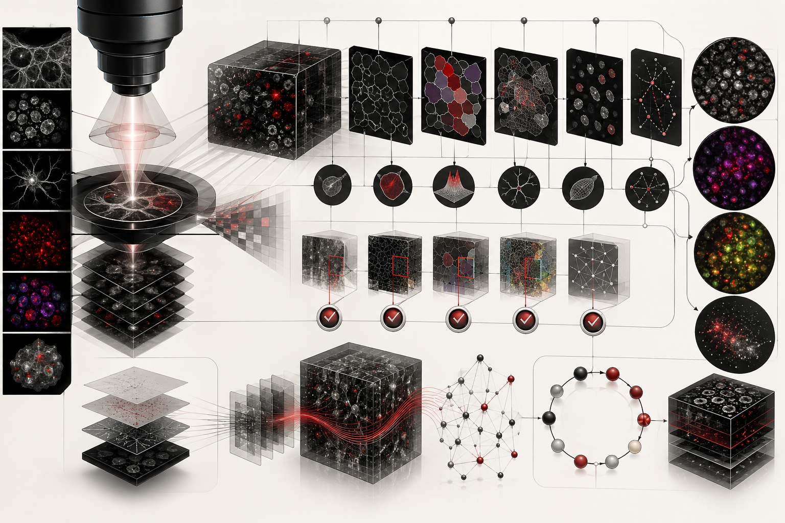
This article introduces microscopy image analysis as a core method in computational biology. It explains how biological images move from specimens to optical systems, from detectors to pixels, from pixels to segmentation masks, from masks to quantitative features, and from features to biological interpretation. The central argument is that images are not merely pictures. They are measurements shaped by optics, sample preparation, illumination, detector response, staining, resolution, noise, metadata, algorithms, and biological assumptions.

The article is written for biologists, cell biologists, developmental biologists, neuroscientists, microbiologists, biomedical researchers, computational biologists, bioimage analysts, laboratory scientists, data engineers, scientific software developers, imaging-core teams, and engineers. It emphasizes image formation, metadata, segmentation, feature extraction, registration, tracking, colocalization, high-content screening, reproducibility, provenance, quality control, and responsible computational interpretation.

The article also extends the discussion into reproducible computational practice through Python and R examples, synthetic microscopy arrays, threshold segmentation, object labeling, intensity-feature extraction, colocalization scaffolds, tracking summaries, SQL-backed provenance, validation metrics, and a linked full-stack GitHub repository containing Python, R, Julia, Fortran, Rust, Go, C, C++, SQL, notebooks, data files, validation notes, and reproducibility documentation.

Why microscopy image analysis matters

Microscopy image analysis matters because much of biology is spatial, visual, and dynamic. Cells change shape. Organelles move. Tissues pattern. Microbes grow. Neurons branch. Embryos develop. Proteins localize. Immune cells migrate. Tumors invade. Plant tissues organize. Biofilms form. These processes cannot be fully understood from tables alone because location, morphology, intensity, adjacency, and movement are biologically meaningful.

Manual visual inspection remains important, especially for discovery, quality control, and expert interpretation. But visual inspection can be subjective, slow, inconsistent, and difficult to scale. Computational image analysis makes microscopy more quantitative by extracting measurable features from images: object count, area, shape, intensity, texture, distance, overlap, motion, branching, neighborhood structure, and spatial organization.

The goal is not to replace biological judgment. The goal is to make image-based evidence more explicit, reproducible, and testable. A segmentation mask can be reviewed. A threshold can be documented. A feature table can be audited. A workflow can be rerun. A model can be compared against ground truth.

Computational microscopy therefore links observation to measurement. It helps scientists ask not only “what do we see?” but “how was it measured, how reliable is the measurement, and what biological claim can it support?”

Back to top ↑

Images as biological measurements

A microscopy image is not a direct copy of biological reality. It is a measurement produced by a specimen, optical system, illumination source, detector, acquisition settings, sample preparation, contrast mechanism, and computational processing pipeline. This matters because every step can shape what appears in the image.

A fluorescent image depends on labeling specificity, fluorophore brightness, photobleaching, illumination uniformity, detector sensitivity, exposure time, background signal, autofluorescence, optical blur, and spectral bleed-through. A brightfield image depends on contrast, staining, focus, thickness, scattering, and sample preparation. Electron microscopy depends on fixation, sectioning, staining, beam conditions, and reconstruction. Light-sheet microscopy, confocal microscopy, super-resolution microscopy, and whole-slide imaging each produce different data structures and artifacts.

Image analysis therefore begins before algorithms. It begins with experimental design and acquisition discipline. Pixel intensities should not be interpreted without understanding how they were generated. Object boundaries should not be trusted without considering resolution, blur, staining, background, and noise. Quantitative comparisons require consistent acquisition or careful normalization.

Biological images become scientific evidence only when acquisition, processing, analysis, and interpretation remain connected.

Back to top ↑

Pixels, voxels, channels, and metadata

Microscopy images are often multidimensional. A simple image may have two spatial dimensions, but biological imaging frequently includes z-stacks, time series, fluorescence channels, fields of view, tiles, regions of interest, wells, plates, samples, and experimental conditions. A pixel represents a measured intensity at a spatial location. A voxel extends this into three dimensions. A channel records intensity for a wavelength, stain, marker, or contrast mode. A time dimension records change.

Metadata are essential because image values are incomplete without context. Pixel size, z-spacing, channel identity, exposure time, objective, numerical aperture, detector gain, acquisition time, illumination settings, microscope type, sample identifier, plate position, and processing history all affect interpretation. Without metadata, two images may look comparable while representing different physical scales or acquisition conditions.

This is why biological image standards matter. Image-analysis workflows should preserve spatial calibration, channel identity, dimensional order, acquisition metadata, and provenance whenever possible. A cell area measured in pixels is less useful than a cell area measured in calibrated physical units. A fluorescence intensity is less interpretable without channel and acquisition context.

In computational biology, metadata are not administrative details. They are part of the measurement.

Back to top ↑

Image quality, resolution, and noise

Image quality determines what can be measured. Resolution affects whether structures can be separated. Signal-to-noise ratio affects whether objects can be detected. Background affects intensity measurement. Blur affects boundary detection. Saturation destroys quantitative information. Uneven illumination can create false spatial patterns. Focus drift can distort time-lapse analysis. Motion artifacts can compromise live imaging. Compression can damage measurements.

Quality control should therefore be explicit. A workflow may assess saturation, intensity range, background level, object count, focus measure, signal-to-noise ratio, channel bleed-through, field illumination, segmentation failure, and outlier images. In high-content imaging, quality control may identify wells or fields that should be excluded. In time-lapse imaging, it may identify frames with drift or focus failure. In whole-slide imaging, it may detect tissue folds, empty regions, or staining artifacts.

Image quality is not a cosmetic issue. It determines the validity of measurement. A beautiful image can be quantitatively unreliable; a visually plain image can be scientifically useful if properly calibrated and analyzed.

Back to top ↑

Segmentation and object detection

Segmentation is the process of assigning pixels or voxels to objects, regions, or background. In microscopy, segmentation may identify nuclei, cells, organelles, tissues, membranes, colonies, plaques, synapses, vessels, fibers, lesions, or microbial clusters. Object detection may identify approximate locations rather than full pixel masks.

Segmentation is often the critical step in image analysis because downstream measurements depend on it. If nuclei are merged, cell counts are wrong. If cell boundaries are too small, intensity measurements are biased. If background is included, texture and morphology features change. If faint objects are missed, biological conclusions may shift.

Segmentation methods include thresholding, edge detection, watershed, region growing, morphology, active contours, graph methods, machine learning, and deep learning. No method is universally correct. The right approach depends on image quality, contrast, object shape, biological question, annotation availability, scale, and validation.

A segmentation workflow should be evaluated. Ground-truth masks, expert review, spot checks, intersection-over-union, Dice coefficient, false positives, false negatives, and failure-case analysis can help determine whether segmentation is adequate for the biological claim.

Back to top ↑

Feature extraction and biological phenotypes

After segmentation, image analysis often extracts features. These may include object count, area, perimeter, circularity, eccentricity, solidity, intensity mean, intensity total, texture, granularity, spot count, distance to boundary, nearest-neighbor distance, branching length, skeleton structure, colocalization, and spatial distribution. In high-content imaging, hundreds or thousands of features may be extracted per cell.

Features are not automatically biological phenotypes. A feature becomes meaningful when connected to biological interpretation. Nuclear area may relate to cell cycle state, but not always. Mitochondrial texture may reflect morphology, but may also reflect staining quality. Fluorescence intensity may approximate abundance, but only under controlled conditions. Shape features may indicate differentiation, stress, migration, or artifact depending on context.

Computational biology therefore requires feature literacy. Researchers should know what each feature measures, how it depends on segmentation, whether it is robust to acquisition variation, whether it is biologically interpretable, and whether it supports the scientific claim.

Feature extraction turns images into tables, but interpretation turns tables into biology.

Back to top ↑

Registration, colocalization, and spatial structure

Many biological questions are spatial. Do two proteins localize together? Does a signal concentrate near the membrane? Do cells cluster around a vessel? Does a tissue region align with a marker? Does an organelle move toward a structure? Does a cell state depend on neighborhood context?

Registration aligns images across channels, time points, fields, or modalities. It may correct drift, align z-stacks, stitch tiles, overlay fluorescence channels, or map microscopy data to tissue coordinates. Poor registration can create false colocalization or obscure real relationships.

Colocalization analysis examines spatial overlap or correlation between signals. It requires caution because overlapping signals can result from optical blur, threshold choice, background, bleed-through, resolution limits, or dense structures. Pearson correlation, Manders coefficients, object-based overlap, distance-based analysis, and spatial-randomization tests each answer different questions.

Spatial structure is central in tissues and communities. Cell neighborhoods, tissue architecture, immune infiltration, microbial biofilms, neural circuits, vascular structure, and developmental patterning all require spatial reasoning. Computational image analysis makes these spatial relationships measurable.

Back to top ↑

Tracking, time-lapse, and dynamic biology

Time-lapse microscopy adds motion and change. Cells divide, migrate, differentiate, die, respond to signals, interact, and reorganize. Organelles move. Proteins assemble and disperse. Embryos develop. Microbes expand. Neural activity changes. Tracking converts image sequences into trajectories.

Tracking typically begins with detection or segmentation in each frame, followed by linking objects across time. Linking can be difficult when objects divide, merge, disappear, overlap, change shape, or move quickly. Tracking errors can distort velocity, displacement, lineage, division timing, persistence, and interaction measurements.

Time-lapse workflows should therefore report tracking quality. They may include track length, gap closing, lineage errors, motion outliers, manual correction, and validation against annotated sequences. For biological interpretation, tracking also requires attention to phototoxicity, photobleaching, environmental conditions, and imaging intervals.

Dynamic biology cannot be captured by static snapshots alone. Computational tracking helps transform image sequences into temporal evidence.

Back to top ↑

High-content screening and image-based profiling

High-content screening uses microscopy to measure large numbers of cells, wells, perturbations, compounds, genes, doses, or time points. It is widely used in cell biology, drug discovery, toxicology, functional genomics, phenotypic screening, organoid analysis, and systems biology. The logic is simple: images contain rich phenotypic information, and computational workflows can extract it at scale.

Image-based profiling often extracts many features per cell and uses statistical or machine-learning methods to compare conditions. A perturbation may change cell morphology, nuclear texture, organelle distribution, cytoskeletal structure, marker localization, or spatial organization. These changes can produce a phenotypic signature.

The strength of high-content analysis is scale and richness. The risk is complexity and artifact. Batch effects, plate position, staining variation, focus differences, segmentation failure, cell-density effects, and feature redundancy can produce misleading results. Experimental design, normalization, controls, replication, and quality control are essential.

High-content microscopy is most powerful when image acquisition, computational analysis, and statistical design are planned together.

Back to top ↑

Deep learning and bioimage analysis

Deep learning has transformed bioimage analysis, especially segmentation, denoising, classification, restoration, super-resolution, object detection, and image-based profiling. Neural networks can learn complex patterns that are difficult to encode manually. They can perform well on challenging microscopy images when trained and validated carefully.

But deep learning requires caution. A model may perform well on images similar to its training data and fail on another microscope, stain, tissue, species, lab, or acquisition protocol. It may learn artifacts rather than biology. It may produce plausible-looking outputs that are not faithful to measured data. It may obscure uncertainty and make failure modes difficult to detect.

Responsible deep-learning use in microscopy requires training-data documentation, annotation quality review, held-out validation, cross-batch testing, uncertainty awareness, failure-case analysis, and biological review. For restoration or denoising, it is especially important to avoid hallucinating structures that were not measured.

Deep learning can be powerful, but it should be integrated into a transparent scientific workflow rather than treated as an automatic source of truth.

Back to top ↑

Reproducibility, provenance, and image data standards

Microscopy workflows can be difficult to reproduce because images are large, multidimensional, metadata-rich, and often stored in proprietary formats. A reproducible project should preserve raw images, acquisition metadata, processing scripts, segmentation masks, feature tables, quality-control reports, parameter settings, software versions, and analysis outputs.

Provenance records how image data were transformed. It answers: which raw image was used, which processing steps were applied, which segmentation parameters were used, which masks were generated, which features were extracted, which objects were excluded, and which plots or tables were produced?

Standards and interoperable formats help. OME-style metadata, OME-TIFF, Bio-Formats, multidimensional image viewers, public bioimage archives, and workflow documentation all support more durable image science. They allow image data to move across tools, labs, repositories, and years.

In computational microscopy, reproducibility is not optional. It is the difference between a visual impression and a scientific measurement system.

Back to top ↑

Mathematical lens: image analysis

Several mathematical ideas are central to microscopy image analysis. These expressions do not replace biological interpretation, but they help clarify how images, masks, signal quality, spatial position, segmentation agreement, colocalization, and tracking can be represented formally.

Image as a function

Threshold segmentation

Signal-to-noise ratio

Convolution

Centroid

Object area

Dice coefficient

Intersection over Union

Pearson colocalization

Tracking displacement

Back to top ↑

Python and R workflows

The following examples are compact article-level workflows. The full GitHub repository expands them into richer full-stack implementations with SQL provenance, synthetic microscopy images, segmentation masks, feature tables, colocalization summaries, tracking scaffolds, validation metrics, and reproducible documentation.

Python example: synthetic microscopy image and threshold segmentation

import math
import pandas as pd

def gaussian_intensity(x, y, cx, cy, sigma, amplitude):
    """Return intensity from a 2D Gaussian object."""
    distance_squared = (x - cx) ** 2 + (y - cy) ** 2
    return amplitude * math.exp(-distance_squared / (2 * sigma ** 2))

objects = [
    {"object_id": "cell_01", "cx": 18, "cy": 20, "sigma": 4.0, "amplitude": 140},
    {"object_id": "cell_02", "cx": 42, "cy": 25, "sigma": 5.0, "amplitude": 170},
    {"object_id": "cell_03", "cx": 30, "cy": 45, "sigma": 4.5, "amplitude": 155},
]

rows = []

for y in range(64):
    for x in range(64):
        intensity = 18.0
        for obj in objects:
            intensity += gaussian_intensity(
                x=x,
                y=y,
                cx=obj["cx"],
                cy=obj["cy"],
                sigma=obj["sigma"],
                amplitude=obj["amplitude"],
            )

        rows.append({"x": x, "y": y, "intensity": intensity})

image = pd.DataFrame(rows)
threshold = 65.0
image["mask"] = image["intensity"] >= threshold

print(image.head().round(3).to_string(index=False))
print("foreground_pixels:", int(image["mask"].sum()))

Python example: object feature extraction from labeled pixels

import pandas as pd

pixels = pd.DataFrame(
    {
        "object_id": ["cell_01"] * 5 + ["cell_02"] * 5,
        "x": [10, 11, 10, 11, 12, 30, 31, 30, 31, 32],
        "y": [10, 10, 11, 11, 11, 20, 20, 21, 21, 21],
        "intensity": [120, 132, 128, 140, 125, 180, 190, 176, 188, 181],
    }
)

features = (
    pixels.groupby("object_id")
    .agg(
        area_pixels=("intensity", "size"),
        mean_intensity=("intensity", "mean"),
        integrated_intensity=("intensity", "sum"),
        centroid_x=("x", "mean"),
        centroid_y=("y", "mean"),
    )
    .reset_index()
)

print(features.round(4).to_string(index=False))

Python example: segmentation agreement metrics

import pandas as pd

comparison = pd.DataFrame(
    {
        "pixel_id": list(range(10)),
        "expert_mask": [1, 1, 1, 1, 0, 0, 0, 1, 0, 0],
        "model_mask":  [1, 1, 0, 1, 0, 1, 0, 1, 0, 0],
    }
)

intersection = ((comparison["expert_mask"] == 1) & (comparison["model_mask"] == 1)).sum()
expert_area = (comparison["expert_mask"] == 1).sum()
model_area = (comparison["model_mask"] == 1).sum()
union = ((comparison["expert_mask"] == 1) | (comparison["model_mask"] == 1)).sum()

dice = 2 * intersection / (expert_area + model_area)
iou = intersection / union

metrics = pd.DataFrame(
    {
        "metric": ["Dice", "IoU"],
        "value": [dice, iou],
    }
)

print(metrics.round(4).to_string(index=False))

Python example: colocalization scaffold

import pandas as pd

pixels = pd.DataFrame(
    {
        "pixel_id": list(range(8)),
        "channel_a": [12, 18, 25, 40, 52, 60, 64, 70],
        "channel_b": [10, 17, 28, 35, 55, 59, 61, 76],
    }
)

pearson = pixels["channel_a"].corr(pixels["channel_b"])

pixels["a_positive"] = pixels["channel_a"] >= 30
pixels["b_positive"] = pixels["channel_b"] >= 30

overlap_fraction = (
    (pixels["a_positive"] & pixels["b_positive"]).sum()
    / max(pixels["a_positive"].sum(), 1)
)

summary = pd.DataFrame(
    {
        "metric": ["pearson_colocalization", "overlap_fraction_a_positive"],
        "value": [pearson, overlap_fraction],
    }
)

print(summary.round(4).to_string(index=False))

Python example: time-lapse tracking summary

import math
import pandas as pd

tracks = pd.DataFrame(
    {
        "track_id": ["track_01", "track_01", "track_01", "track_02", "track_02", "track_02"],
        "frame": [0, 1, 2, 0, 1, 2],
        "x": [10.0, 12.5, 15.0, 30.0, 30.8, 32.2],
        "y": [10.0, 11.0, 13.0, 20.0, 22.1, 24.5],
    }
)

rows = []

for track_id, subset in tracks.sort_values(["track_id", "frame"]).groupby("track_id"):
    subset = subset.reset_index(drop=True)

    total_distance = 0.0
    for i in range(len(subset) - 1):
        dx = subset.loc[i + 1, "x"] - subset.loc[i, "x"]
        dy = subset.loc[i + 1, "y"] - subset.loc[i, "y"]
        total_distance += math.sqrt(dx ** 2 + dy ** 2)

    displacement = math.sqrt(
        (subset.loc[len(subset) - 1, "x"] - subset.loc[0, "x"]) ** 2
        + (subset.loc[len(subset) - 1, "y"] - subset.loc[0, "y"]) ** 2
    )

    rows.append(
        {
            "track_id": track_id,
            "frames": len(subset),
            "total_distance": total_distance,
            "net_displacement": displacement,
        }
    )

summary = pd.DataFrame(rows)

print(summary.round(4).to_string(index=False))

R example: threshold segmentation cross-check

# Compact R threshold segmentation cross-check.

image_pixels <- data.frame(
  pixel_id = 1:10,
  intensity = c(18, 22, 35, 68, 91, 110, 74, 42, 20, 15)
)

threshold <- 65
image_pixels$mask <- image_pixels$intensity >= threshold

foreground_pixels <- sum(image_pixels$mask)
mean_foreground_intensity <- mean(image_pixels$intensity[image_pixels$mask])

summary_table <- data.frame(
  threshold = threshold,
  foreground_pixels = foreground_pixels,
  mean_foreground_intensity = mean_foreground_intensity
)

print(round(summary_table, 4))

Back to top ↑

GitHub repository

The article body includes compact Python and R examples so the scientific argument remains readable. The full repository expands those examples into a rigorous workflow for image analysis, microscopy, and computational biology, including synthetic microscopy image generation, threshold segmentation, connected-component scaffolds, object feature extraction, segmentation validation, colocalization analysis, tracking summaries, metadata tables, SQL provenance, notebook documentation, cross-language validation helpers, and full-stack scientific-computing examples across Python, R, Julia, Fortran, Rust, Go, C, C++, SQL, and notebooks.

Back to top ↑

Limits, ethics, and responsible interpretation

Computational image analysis can make microscopy more quantitative, but it can also produce misleading precision. A segmentation mask may look objective while encoding threshold bias. A feature table may contain thousands of measurements that depend on imperfect object boundaries. A deep-learning model may perform well on familiar images and fail on another microscope, tissue, stain, or lab. A denoising model may create visually convincing structures that were not reliably measured.

Ethics also matter. Biomedical images can contain patient-derived material, clinical context, or identifiable metadata. Human tissue imaging, pathology, developmental imaging, and clinical microscopy require governance, consent, privacy protection, and careful communication. Algorithmic errors may affect downstream biological claims, diagnostic research, or resource allocation. Public image archives expand scientific value, but they also require responsible data stewardship.

Responsible microscopy image analysis requires acquisition discipline, metadata preservation, validation, uncertainty communication, expert review, reproducible workflows, and humility about what images can prove.

Back to top ↑

Why computational microscopy matters today

Computational microscopy matters today because biology is increasingly image-rich. Modern instruments generate large, multidimensional, high-resolution datasets. Single-cell imaging, organoids, spatial biology, high-content screens, tissue atlases, developmental imaging, live-cell microscopy, pathology, super-resolution imaging, and electron microscopy all require computational methods to make images interpretable at scale.

Image analysis also connects biology to engineering. It requires optics, sensors, signal processing, statistics, computer vision, machine learning, data management, software engineering, and scientific visualization. This makes computational microscopy a bridge between laboratory biology and scientific infrastructure.

The deeper value is not automation alone. It is accountable measurement. Computational image analysis helps scientists turn visual evidence into documented, reviewable, reproducible, and biologically meaningful data.

Back to top ↑

Conclusion

Image analysis, microscopy, and computational biology provide a rigorous framework for studying living systems through visual measurement. Microscopy reveals cells, tissues, structures, signals, and dynamics. Computational workflows transform those images into masks, features, trajectories, spatial relationships, quality-control reports, and reproducible evidence.

The strongest image-analysis workflows are not the most complex. They are the clearest about acquisition, metadata, segmentation, validation, feature meaning, uncertainty, and biological interpretation. They preserve the connection between image formation and scientific claim.

Used responsibly, computational microscopy does not reduce living systems to pixels. It helps make visual biology measurable, auditable, and scientifically trustworthy.

Back to top ↑

Related articles

• Biology
• Cell Structure, Membranes, and Organelles
• Molecular Biology and the Flow of Genetic Information
• Data, Measurement, and Reproducibility in the Life Sciences
• Python for Simulation, Bioinformatics, and Scientific Workflows
• Python for Biological Modeling and Automation
• R for Biological Data Analysis and Visualization
• Statistics, Uncertainty, and Measurement in Biology
• Biostatistics and Experimental Design in Biology
• Networks, Systems, and Biological Complexity
• Genomics, Sequence Analysis, and Biological Data

Further reading

• Open Microscopy Environment (2022) The OME-TIFF Format. Available at: https://docs.openmicroscopy.org/ome-model/6.3.1/ome-tiff/index.html
• Open Microscopy Environment (2020) OME Data Model and File Formats. Available at: https://docs.openmicroscopy.org/ome-model/6.2.2/
• Bio-Formats (2025) ImageJ Overview. Available at: https://bio-formats.readthedocs.io/en/v8.1.1/users/imagej/
• CellProfiler (n.d.) CellProfiler. Available at: https://cellprofiler.org/
• CellProfiler Documentation (n.d.) Welcome to CellProfiler’s Documentation. Available at: https://cellprofiler-manual.s3.amazonaws.com/CellProfiler-4.2.6/index.html
• napari (n.d.) napari: A Fast, Interactive Viewer for Multi-Dimensional Images in Python. Available at: https://napari.org/
• scikit-image Developers (n.d.) scikit-image Documentation. Available at: https://scikit-image.org/docs/stable/
• BioImage Archive (n.d.) BioImage Archive. Available at: https://www.ebi.ac.uk/bioimage-archive/
• Image Data Resource (n.d.) Image Data Resource. Available at: https://idr.openmicroscopy.org/
• National Institutes of Health (n.d.) ImageJ. Available at: https://imagej.nih.gov/ij/

References

• Bio-Formats (2025) ImageJ Overview. Available at: https://bio-formats.readthedocs.io/en/v8.1.1/users/imagej/
• BioImage Archive (n.d.) BioImage Archive. Available at: https://www.ebi.ac.uk/bioimage-archive/
• CellProfiler (n.d.) CellProfiler. Available at: https://cellprofiler.org/
• CellProfiler Documentation (n.d.) Welcome to CellProfiler’s Documentation. Available at: https://cellprofiler-manual.s3.amazonaws.com/CellProfiler-4.2.6/index.html
• Image Data Resource (n.d.) Image Data Resource. Available at: https://idr.openmicroscopy.org/
• napari (n.d.) napari: A Fast, Interactive Viewer for Multi-Dimensional Images in Python. Available at: https://napari.org/
• National Institutes of Health (n.d.) ImageJ. Available at: https://imagej.nih.gov/ij/
• Open Microscopy Environment (2020) OME Data Model and File Formats. Available at: https://docs.openmicroscopy.org/ome-model/6.2.2/
• Open Microscopy Environment (2022) The OME-TIFF Format. Available at: https://docs.openmicroscopy.org/ome-model/6.3.1/ome-tiff/index.html
• scikit-image Developers (n.d.) scikit-image Documentation. Available at: https://scikit-image.org/docs/stable/

Back to top ↑