
Last Updated May 11, 2026
Robotics, actuation, and physical feedback loops examine how embedded systems transform sensing, estimation, control, and mechanical response into coordinated physical behavior. At a technical level, robotics is not simply software attached to machines, and actuation is not merely output. Robotics is a cyber-physical systems discipline in which kinematics, dynamics, sampling, feedback, state estimation, actuator limits, safety constraints, and real-time execution determine whether computation can produce reliable motion in the physical world.
Robotics matters because embedded decisions become physical consequences. A sensing error can become a motion error. A timing delay can become instability. An actuator saturation limit can turn a valid controller into a poor physical response. A planner may generate a feasible path in software, while the real robot fails because of torque limits, backlash, compliance, latency, calibration drift, contact uncertainty, or insufficient observability of the actual physical state.
The deeper architectural question is therefore not simply how to move a robot, but how to maintain a trustworthy loop between perception, estimation, planning, control, actuation, and physical feedback. A strong robotic system does not merely issue commands. It models physical constraints, estimates state under uncertainty, computes bounded actions, verifies motion through feedback, and transitions to safe behavior when sensing, timing, actuation, or trust conditions degrade.
Main Library
Publications
Article Map
Embedded & Edge Systems
Related Topic
Artificial Intelligence Systems
Related Topic
Intelligent Infrastructure Systems
Related Topic
Environmental Monitoring Systems
For engineering teams, robotics sits at the intersection of embedded systems, control theory, mechanics, electrical design, real-time software, perception, safety engineering, and operational monitoring. A robot becomes dependable only when its cyber layer and physical layer remain synchronized: the controller must act on a valid estimate of the physical state, the actuator must realize commands within physical limits, and the feedback loop must detect when the real system diverges from intended behavior.
Engineering Problem
The engineering problem is how to make embedded computation produce reliable physical behavior under uncertainty, delay, constraint, and disturbance. A robotic system must sense the world, estimate state, plan or track a goal, compute a control action, drive actuators, observe the resulting motion, and correct error continuously. Every part of that loop can fail: sensors can be noisy, estimates can drift, commands can arrive late, actuators can saturate, mechanical systems can flex, and feedback can become unstable.
In software-only systems, incorrect state may cause incorrect output. In robotics, incorrect state can cause unsafe movement. The robot’s correctness is therefore not only logical. It is temporal, mechanical, electrical, and physical. A command may be correct in code but unsafe or ineffective if it arrives too late, exceeds torque limits, ignores contact, violates a safety envelope, or assumes a state estimate that no longer describes the physical system.
Production robotic systems require explicit engineering around control loops, actuator capabilities, sensor timing, bus latency, task scheduling, safety envelopes, failure states, and observability. Engineers need to know not only what the robot is commanded to do, but whether the physical system can realize that command, whether feedback confirms the intended motion, and what happens when it cannot.
This is why robotics is a powerful example of cyber-physical systems engineering. The robot is not simply executing code. It is participating in a feedback relationship with the physical world.
Reference Architecture
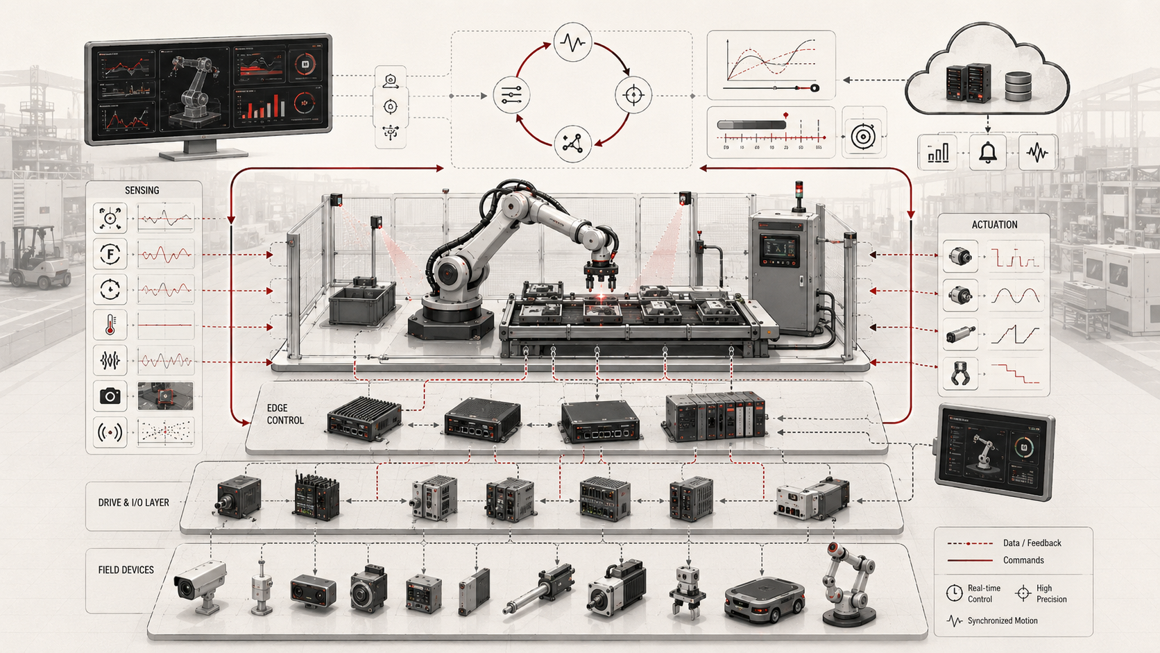
A practical robotic feedback architecture can be understood as a layered loop from sensing to actuation and back again. The specific platform may be a manipulator, mobile robot, drone, autonomous vehicle, inspection robot, warehouse system, surgical robot, or industrial cell, but the engineering pattern is broadly consistent.
| Layer | Engineering Role | Robotics Concern | Evidence Artifact |
|---|---|---|---|
| Sensor layer | Measures joint position, velocity, force, torque, proximity, vision, inertial motion, contact, or environment | Noise, delay, sampling rate, calibration, synchronization, missing data | Sensor profile, calibration record, sampling policy, telemetry schema |
| State-estimation layer | Converts measurements into motion-relevant state | Pose, velocity, contact state, uncertainty, latency compensation, observability | Estimator configuration, covariance log, state-vector schema |
| Planning layer | Defines trajectories, tasks, waypoints, or goals | Feasibility, collision constraints, timing assumptions, dynamic limits | Trajectory plan, task manifest, workspace constraints |
| Control layer | Computes actuator commands from reference and estimated state | Tracking error, stability, saturation, robustness, gain tuning | Controller configuration, gain file, control-loop log |
| Actuation layer | Converts control signals into force, torque, motion, pressure, or displacement | Torque limits, bandwidth, backlash, compliance, thermal behavior, power limits | Actuator profile, motor-driver config, torque/current logs |
| Embedded runtime layer | Schedules control tasks, bus communication, safety checks, telemetry, and watchdogs | Latency, jitter, priority inversion, bus timing, hard real-time behavior | Runtime manifest, timing log, watchdog record |
| Safety and governance layer | Constrains behavior under faults, uncertainty, human proximity, or degraded trust | Safe state, force limits, emergency stop, fallback behavior, compliance | Safety envelope, fault policy, hazard log, validation report |
| Edge coordination layer | Coordinates robots, cells, fleets, gateways, cloud services, and supervisory control | Distributed state, coordination delay, partial failure, shared workspace conflict | Fleet policy, coordination log, edge-control manifest |
This architecture shows why robotics cannot be reduced to either software or hardware alone. The behavior emerges from the loop. Sensors, estimators, controllers, actuators, timing, safety constraints, mechanical structure, and runtime scheduling all shape the final physical outcome.
Implementation Pattern
A practical robotics implementation pattern begins by defining the control loop explicitly. Engineers should identify the controlled variables, measured variables, estimated state, actuator command, sampling period, timing tolerance, actuator limits, safety bounds, and fault behavior before the system is treated as deployment-ready.
A rigorous implementation should include:
| Artifact | Purpose | Typical Format |
|---|---|---|
| Robot profile | Defines robot class, joints, actuators, sensors, power limits, workspace limits, runtime assumptions | JSON or YAML |
| Plant model | Represents physical dynamics, state variables, inputs, outputs, disturbances, and constraints | Python model, MATLAB/Simulink model, URDF/SDF, JSON/YAML metadata |
| Actuator profile | Defines torque, speed, current, travel, resolution, backlash, thermal, and saturation limits | JSON, YAML, datasheet-derived table |
| Sensor calibration record | Defines offsets, scale factors, units, timestamps, uncertainty, and calibration date | CSV, JSON, SQL table |
| Controller configuration | Defines gains, sampling period, target variables, anti-windup behavior, saturation handling, fallback mode | YAML, TOML, JSON, firmware constants |
| Estimator configuration | Defines state vector, observation model, process noise, measurement noise, filtering method, update rate | YAML, JSON, Python config |
| Trajectory manifest | Defines waypoints, velocity limits, acceleration limits, timing, task goals, and workspace constraints | YAML, JSON, ROS-style message, CSV |
| Safety envelope | Defines force limits, speed limits, workspace boundaries, stop conditions, degraded modes, human-proximity rules | YAML, safety case, PLC policy, runtime config |
| Control-loop log | Records setpoint, measured state, estimated state, tracking error, command output, latency, saturation, and fault state | CSV, SQL, telemetry stream, binary log |
| Validation suite | Tests timing, stability, tracking, saturation, estimator failure, actuator fault, and safe-state transition | Python, pytest, Bash, hardware-in-the-loop scripts |
The implementation goal is to make physical behavior testable. A robot should not merely appear to move correctly in a demonstration. Engineers should be able to inspect tracking error, state-estimation quality, timing jitter, actuator saturation, safety-state transitions, and recovery behavior under realistic disturbances and degraded conditions.
Formal Robotics Model: State, Control, Dynamics, and Observation
A more rigorous robotics architecture begins with a formal model of the system being controlled. At a high level, the robot can be represented by a state vector, a control input, an output or observation, and dynamics that describe how the physical state evolves over time.
x_{k+1} = f(x_k, u_k, w_k)
\]
Interpretation: \(x_k\) is the system state at time step \(k\), \(u_k\) is the control input, and \(w_k\) represents process disturbance or model uncertainty. The function \(f\) describes how the robot’s physical state evolves.
y_k = h(x_k, v_k)
\]
Interpretation: \(y_k\) is the measured output, and \(v_k\) represents measurement noise. The function \(h\) describes how the robot’s internal state becomes observable through sensors.
This distinction matters because robotic systems rarely observe their true state directly. Encoders, IMUs, cameras, force sensors, proximity sensors, current sensors, and external tracking systems provide partial, noisy, delayed, and sometimes contradictory measurements. A robot’s controller often acts not on the true state \(x_k\), but on an estimated state \(\hat{x}_k\).
A rigorous architecture therefore asks three questions. First, what state must be controlled? Second, what measurements are available to estimate that state? Third, what inputs can the actuator system actually realize? If any of these answers are vague, the robot may work in limited demonstrations while failing under realistic conditions.
Kinematics, Dynamics, and Physical Feasibility
Robotics depends on both kinematics and dynamics. Kinematics describes geometric relationships: joint angles, link lengths, end-effector pose, wheel velocities, body frames, transformations, and coordinate systems. Dynamics describes the relationship among mass, inertia, forces, torques, acceleration, friction, compliance, and external disturbance.
A motion plan can be kinematically valid while dynamically infeasible. A trajectory may place an end effector at the correct pose while demanding torque, acceleration, grip force, or braking behavior the physical system cannot provide. This distinction is essential in embedded robotics because controllers must operate under real actuator, power, timing, and mechanical constraints.
M(q)\ddot{q} + C(q,\dot{q})\dot{q} + g(q) = \tau
\]
Interpretation: A simplified manipulator dynamics equation relates joint positions \(q\), joint velocities \(\dot{q}\), joint accelerations \(\ddot{q}\), inertia \(M(q)\), velocity-dependent effects \(C(q,\dot{q})\dot{q}\), gravity \(g(q)\), and applied joint torques \(\tau\). Real systems may also include friction, compliance, contact forces, and actuator saturation.
For engineers, this equation is less important as a symbolic ideal than as a reminder that motion has physical cost. If a controller commands \(\tau\) beyond what motors, drives, gears, thermal limits, or power electronics can provide, the robot will not track the intended trajectory. The failure may appear in software as tracking error, but the root cause is physical infeasibility.
Good robotic engineering therefore connects planning to dynamics. Trajectories should respect velocity, acceleration, jerk, torque, workspace, collision, and safety constraints. Controllers should account for saturation and uncertainty. Logs should record whether the robot’s physical system was asked to do something it could not actually do.
Actuation as Physical Interface and Constraint
Actuation is often described as output, but in robotics it is better understood as a constrained physical interface. Motors, servos, valves, drives, grippers, pneumatic systems, hydraulic systems, and end effectors do not carry out commands transparently. They realize commands within physical limits involving speed, torque, resolution, backlash, saturation, thermal behavior, compliance, energy availability, and wear.
This means actuation is part of the architecture of meaning. A control signal only matters insofar as the actuation chain can realize it safely and predictably. A mathematically elegant control law may perform poorly if the actuator bandwidth is too low, if the drivetrain introduces delay or compliance, if the power electronics cannot sustain demanded behavior, or if the mechanism reaches saturation.
For engineers, actuator metadata should be treated as configuration, not folklore. Torque limits, current limits, thermal limits, update rates, encoder resolution, backlash, gear ratios, dead zones, and saturation behavior should be documented and used by planning, control, testing, and safety systems.
Actuation also creates safety obligations. A system with greater torque or speed authority requires stronger constraints, faster safety response, better fault detection, and more careful validation. In robotics, actuator capability is not only a performance property. It is also a risk property.
Feedback Loops and Closed-Loop Robotic Behavior
Physical feedback loops are what make robotic systems responsive rather than merely preprogrammed. The robot observes some aspect of its state or environment, compares that state with a target or policy, computes an action, and applies the action through the actuation layer. The next observation reflects the consequences of that action, and the loop repeats.
This loop may exist at multiple levels. At a low level, motor control loops regulate current, velocity, or position. At a higher level, task controllers coordinate end-effector movement, grasping behavior, or collision avoidance. At still higher levels, mission logic may alter goals, change modes, or reassign subtasks based on the evolving environment.
Strong robotic design distinguishes between open-loop commands and genuine feedback behavior. A robot that only plays out motion scripts under static assumptions is less robust than one that can continually correct itself through sensing and control.
For engineers, feedback loops should be measured. Tracking error, loop frequency, command delay, estimator delay, overshoot, settling time, saturation frequency, disturbance rejection, and recovery behavior are not academic variables. They are operational signals that reveal whether the robot is actually controlling the physical system it claims to control.
State Estimation, Observability, and Sensor Fusion
Robotic systems depend on estimated state. A manipulator may need joint positions, joint velocities, end-effector pose, contact state, and force estimates. A mobile robot may need pose, velocity, terrain, obstacle state, and localization confidence. A collaborative robot may need human proximity, force interaction, and workspace occupancy under uncertainty.
Because measurements are incomplete and noisy, the robot must infer state from observations. This is where observability becomes central. If the sensors do not provide enough information to reconstruct the state needed for control, the system may behave confidently while being physically ignorant.
\hat{x}_{k+1} = A\hat{x}_k + Bu_k + L(y_k – C\hat{x}_k)
\]
Interpretation: This simplified observer form updates the estimated state \(\hat{x}\) using system dynamics \(A\), control input \(B u_k\), measurement \(y_k\), observation matrix \(C\), and correction gain \(L\). The term \(y_k – C\hat{x}_k\) is the innovation: the difference between what the system expected to observe and what it actually measured.
For engineers, estimator behavior should be visible. State estimates should carry units, timestamps, freshness, uncertainty where appropriate, and provenance. When a controller acts on stale, noisy, or overconfident state estimates, the resulting motion error can look like a control problem when the deeper issue is sensing and estimation quality.
Sensor fusion should also be designed with failure behavior. If a camera drops frames, an encoder slips, an IMU drifts, or a force sensor saturates, the robot should not continue treating the fused state as equally trustworthy. State estimation is not only a mathematical layer. It is a trust layer for physical behavior.
Planning, Trajectory Generation, and Control Realization
Robotics depends on multiple layers of decision and control. Planning determines what should be attempted. Trajectory generation converts goals into time-parameterized motion. Control determines how desired behavior should be realized in the presence of disturbance and changing conditions. Motor-level realization determines whether that control intent can actually be executed by the mechanical and electrical system.
This layered structure matters because elegant planning alone does not guarantee good robotic behavior. A path planner may produce a collision-free trajectory that still fails if low-level control cannot track it, if the actuators cannot realize the required motion profile, if timing assumptions are violated, or if the robot encounters contact conditions the planner did not represent.
More advanced robotic systems may use model predictive control, impedance control, admittance control, hybrid force-position control, or optimization-based planning. These methods can improve behavior when the system model, constraints, and timing assumptions are credible. They can also fail if the model is wrong, the solver is too slow, or the resulting commands exceed physical capability.
For engineers, the practical principle is simple: planning must respect control and actuation limits. A planner that ignores acceleration limits, torque limits, joint limits, contact constraints, actuator bandwidth, or safety envelopes is not truly robot-aware. It is producing paths that may be formally valid but physically unrealistic.
Sampled-Data Control, Timing, Latency, and Jitter
Timing is especially unforgiving in robotics because physical motion unfolds continuously while computation unfolds discretely. A command that is correct in principle may be wrong in practice if it arrives too late. A sensor update that is accurate but delayed may cause the robot to act on a world that has already changed.
This is why latency, jitter, scheduling, and synchronization matter so much in robotic systems. Motion correctness depends not only on what the controller computes, but when it computes it relative to the evolving physical state of the mechanism and its environment.
Good architecture identifies which loops are hard-real-time, which are latency-sensitive, and which can tolerate more delay. A motor-current loop may need much tighter timing than a supervisory fleet scheduler. A safety stop may require deterministic response. A high-level planner may tolerate more asynchronous computation. A cloud-connected analytics system may be useful for monitoring but inappropriate for direct high-speed control.
t_{\mathrm{loop}} = t_{\mathrm{sense}} + t_{\mathrm{estimate}} + t_{\mathrm{compute}} + t_{\mathrm{communicate}} + t_{\mathrm{actuate}}
\]
Interpretation: Total loop time includes sensing, estimation, computation, communication, and actuation delay. Robotic correctness depends on whether this loop time and its jitter remain within the stability and safety requirements of the physical system.
Without temporal discipline, robotics can appear algorithmically sophisticated while remaining operationally brittle. Engineers should treat timing as a design constraint, a test target, and an observability signal.
Stability, Safety Envelopes, and Control Barrier Thinking
A robot must not only move. It must remain stable and safe while moving. Stability asks whether the system’s behavior remains bounded and converges toward intended behavior. Safety asks whether the system avoids unacceptable states: collision, excessive force, workspace violation, overheating, loss of control, or operation under invalid sensor assumptions.
Classical control often reasons about stability using Lyapunov-style arguments. The basic idea is to define an energy-like function that should decrease as the system approaches desired behavior.
V(e_k) \geq 0,\qquad V(e_{k+1}) – V(e_k) \leq 0
\]
Interpretation: \(V(e_k)\) is a nonnegative function of tracking error. If \(V\) does not increase over time, the system is moving toward more stable behavior under the assumptions of the model. Real robotic systems must still account for saturation, delay, unmodeled dynamics, and disturbance.
Modern safety-oriented control often represents safe behavior as a constraint on the system state. A safety function \(h(x)\) can define a safe set where \(h(x) \geq 0\). The controller should choose actions that keep the system inside that safe set.
h(x_k) \geq 0
\]
Interpretation: The condition \(h(x_k) \geq 0\) means the robot’s state is inside the defined safe region. Examples include staying outside a human-proximity zone, within workspace boundaries, below force limits, or below thermal thresholds.
For engineers, these concepts should not remain abstract. Safety envelopes should be represented in configuration and tested under realistic conditions. The robot should know when it is approaching a boundary, when it must slow down, when it must stop, when it must degrade behavior, and when operator intervention is required.
Safety is therefore not a separate layer after control. It is a constraint on control, planning, actuation, runtime scheduling, sensing, estimation, and operations.
Mechanical, Electrical, and Embedded Integration
Robotics is often described through software stacks, but the physical system is equally important. Mechanical compliance, gearing, backlash, bearing quality, wiring, bus architecture, motor drivers, power delivery, thermal limits, and embedded timing all shape what the robot can actually do.
This means robotic performance emerges from integration across layers. A robot may fail not because the control logic is weak, but because the wiring introduces noise, the gear train introduces slack, the communication bus adds jitter, the power supply droops under load, or the thermal profile degrades actuator performance over time.
Good design treats mechanics, electronics, and embedded computation as one coupled system rather than as separable teams handing work off linearly. In robotics, integration quality often matters as much as algorithmic sophistication.
For engineers, integration testing should include realistic load, duty cycles, environmental conditions, motion profiles, communication patterns, and power states. A robot that works on a bench may fail in a cell, warehouse, field site, hospital, laboratory, or shared workspace because the physical integration assumptions were never tested under realistic conditions.
Distributed Robotics and Coordinated Physical Systems
Many robotic systems are distributed rather than isolated. A production cell may include multiple arms, conveyors, drives, sensors, safety systems, vision stations, and edge gateways. A warehouse fleet may coordinate many mobile robots. A field system may combine local robot control with edge infrastructure, supervisory coordination, and remote monitoring.
This makes communication part of robotic behavior rather than just a logging or management feature. Delayed coordination messages, inconsistent beliefs about shared state, or partial subsystem failure can affect physical behavior directly.
Good distributed robotics design limits hidden dependence on perfectly synchronized global knowledge. It defines what each subsystem can decide locally, what requires coordination, and how disagreement or temporary separation is handled without making the whole system unsafe or unusable.
For engineers, distributed robotics requires explicit contracts around timing, ownership, shared state, message freshness, command authority, safety precedence, and fallback behavior. A robot fleet is not just many robots. It is a coordinated physical system with distributed control and distributed failure modes.
Data and Configuration Artifacts
Robotic systems become easier to test, tune, and govern when their assumptions are represented as data and configuration artifacts. Engineers should be able to inspect actuator limits, control-loop settings, sensor calibration, safety envelopes, timing budgets, trajectory constraints, estimator assumptions, and failure-state policies without relying only on undocumented code or operator memory.
| Artifact | What It Captures | Engineering Purpose |
|---|---|---|
robot_profile.json |
Robot type, joints, sensors, actuators, power constraints, workspace limits, runtime assumptions | Defines the physical system being controlled |
plant_model.py |
State variables, dynamics, inputs, outputs, disturbances, and constraints | Supports simulation, controller design, and validation |
actuator_profile.yml |
Torque, speed, current, thermal, backlash, saturation, and resolution limits | Prevents physically unrealistic commands |
sensor_calibration.csv |
Offsets, scale factors, units, calibration date, uncertainty notes | Supports trustworthy state estimation and repeatable measurement |
estimator_config.yml |
State vector, observation model, noise assumptions, filter gains, update rate | Makes estimation behavior reviewable and tunable |
controller_config.yml |
Control gains, sampling period, target variables, saturation handling, fallback mode | Makes controller behavior reviewable and reproducible |
safety_envelope.yml |
Force limits, speed limits, workspace boundaries, emergency-stop rules, degraded modes | Defines safe operating boundaries |
trajectory_manifest.json |
Waypoints, timing, velocity limits, acceleration limits, task goals, constraints | Connects planning to physical feasibility |
control_loop_log.csv |
Setpoint, measured state, estimated state, tracking error, command output, latency, saturation, fault state | Enables debugging, tuning, validation, and incident review |
robotics_event_schema.sql |
Tables for motion events, control errors, actuator states, faults, and safety transitions | Makes robotic behavior queryable and auditable |
The goal is not to force one robotics framework or file format. The goal is to make the physical assumptions explicit enough that control behavior can be tested, compared, tuned, monitored, and improved over time.
Mathematical Lens: State-Space Feedback, Tracking Error, and Safety Constraints
A technical robotics lens begins with state, control, and feedback. In discrete time, a simplified linear state-space model can be written as:
x_{k+1} = Ax_k + Bu_k + w_k
\]
Interpretation: \(x_k\) is the robot state, \(u_k\) is the actuator command, \(A\) represents the system dynamics, \(B\) maps commands into state change, and \(w_k\) represents disturbance or model uncertainty.
y_k = Cx_k + v_k
\]
Interpretation: \(y_k\) is the measured output, \(C\) maps state into measurement, and \(v_k\) represents sensor noise. The controller often acts on an estimated state rather than the true state.
A feedback controller may then compute a command from tracking error:
e_k = r_k – y_k
\]
Interpretation: \(e_k\) is the tracking error at time step \(k\), \(r_k\) is the reference or desired state, and \(y_k\) is the measured or estimated output.
u_k = K_p e_k + K_i \sum_{j=0}^{k} e_j \Delta t + K_d \frac{e_k – e_{k-1}}{\Delta t}
\]
Interpretation: This PID-style controller computes actuator command \(u_k\) from proportional, integral, and derivative terms. In real robotic systems, \(u_k\) must also respect actuator saturation, sampling period, timing jitter, safety limits, and mechanical dynamics.
For safety-critical motion, the command should also preserve a safe set:
h(x_k) \geq 0
\]
Interpretation: \(h(x_k)\) defines a safety condition. The robot remains inside the safe region when this condition is satisfied. Safety functions can represent workspace boundaries, distance from humans, force limits, temperature limits, or collision constraints.
The key engineering point is that robotics math must be connected to implementation. A controller is not only a formula. It is a sampled, delayed, saturated, noisy, constrained, and physically realized feedback process. Tracking error, command output, saturation, loop timing, settling time, overshoot, disturbance recovery, and safety-envelope violations should be logged and analyzed.
Python Workflow: State-Space Feedback Simulation with Saturation, Delay, and Jitter
The companion Python workflow should model a simplified robotic control loop using state-space dynamics, tracking error, actuator saturation, timing jitter, and disturbance. The goal is to show how engineers can turn feedback-loop concepts into reproducible analysis rather than leaving motion quality as subjective observation.
# Python Workflow: State-Space Feedback Simulation with Saturation, Delay, and Jitter

error = reference_position - measured_position

integral_error += error * dt
derivative_error = (error - previous_error) / dt

raw_command = (
    kp * error
    + ki * integral_error
    + kd * derivative_error
)

command = max(min(raw_command, actuator_limit), -actuator_limit)
saturated = command != raw_command

next_state = A @ state + B.flatten() * command + disturbance
This workflow is useful for testing control assumptions before deploying them into firmware or real robotic hardware. It can be adapted to evaluate tracking error, saturation behavior, loop frequency, overshoot, settling time, noise sensitivity, delay sensitivity, and disturbance recovery.
For production robotics, the same workflow can be connected to real control logs from embedded devices, motor controllers, edge runtimes, robotic middleware, or fielded robots. Engineers can then compare commanded behavior against measured behavior and identify whether failures come from controller tuning, timing jitter, actuator limits, sensor delay, estimator quality, or mechanical integration.
R Workflow: Actuator Performance, Tracking Error, and Reliability Reporting
The companion R workflow focuses on reporting. It should summarize tracking error, actuator saturation, timing jitter, fault frequency, recovery behavior, and performance differences across robot units, joints, tasks, or operating modes. Where Python is useful for simulation and control-loop analysis, R is useful for fleet-level reporting, reliability summaries, quality analysis, and engineering review tables.
# R Workflow: Actuator Performance, Tracking Error, and Reliability Reporting

robotics_summary <- control_logs |>
  dplyr::group_by(robot_id, joint_id, task_mode) |>
  dplyr::summarise(
    mean_abs_error = mean(abs(tracking_error), na.rm = TRUE),
    max_abs_error = max(abs(tracking_error), na.rm = TRUE),
    saturation_rate = mean(saturated, na.rm = TRUE),
    mean_loop_jitter_ms = mean(loop_jitter_ms, na.rm = TRUE),
    safety_events = sum(safety_state != "normal", na.rm = TRUE),
    faults = sum(fault_state != "normal", na.rm = TRUE),
    .groups = "drop"
  )
This workflow helps engineering teams distinguish isolated failures from systematic design issues. If one actuator saturates often, that may suggest undersizing or poor tuning. If one robot has higher jitter, the issue may be runtime scheduling or communication. If one task mode produces high tracking error, the trajectory may exceed physical capability.
For robotic systems deployed across fleets, cells, or sites, reporting is essential. Physical systems degrade. Actuators wear. Calibration drifts. Timing changes after software updates. Reporting turns those changes into visible engineering evidence.
Systems Code: Firmware, Control Loops, MicroPython, TinyML, PYNQ, HDL, Bash, and Configuration
The companion repository should be useful to engineers because robotics crosses the full embedded and edge stack. It touches firmware, motor-control logic, gateway coordination, simulation, reporting, timing analysis, safety envelopes, constrained inference, FPGA-backed acceleration, HDL control blocks, and repeatable workflow scripts.
| Folder | Engineering Role | Robotics Use |
|---|---|---|
python/ |
Simulation and workflow automation | State-space simulation, feedback-loop analysis, saturation modeling, jitter sensitivity |
r/ |
Reporting and descriptive analytics | Actuator performance summaries, tracking-error analysis, safety-event reporting |
sql/ |
Queryable engineering evidence | Stores robot state, control logs, actuator events, faults, and safety transitions |
c/ |
Constrained embedded control | PID loop, motor command bounds, watchdog checks, real-time actuator updates |
cpp/ |
Robotics middleware and gateway abstractions | State machines, command validation, trajectory execution, controller interfaces |
rust/ |
Safe systems validation | Safety-envelope validation, command-bound checking, state transition rules |
go/ |
Operational services and fleet utilities | Robot telemetry gateway, coordination service, control-event router |
micropython/ |
Microcontroller prototypes | Servo control, sensor reading, local feedback-loop demonstration |
tinyml/ |
Constrained local inference | Fault detection, vibration anomaly detection, contact-state classification |
pynq/ |
FPGA-backed acceleration | Low-latency signal filtering, encoder preprocessing, trajectory acceleration |
hdl/ |
Hardware/software co-design | PWM scaffolds, quadrature encoder logic, stream filters, hardware timing gates |
bash/ |
Repeatable workflow execution | Runs simulations, validates manifests, generates output summaries |
config/ |
Machine-readable robotics metadata | Robot profiles, actuator profiles, controller settings, estimator configs, safety envelopes |
This cross-layer stack matters because robotic performance is not created by one component. The same design concern appears in firmware, mechanical limits, control math, telemetry, safety policy, data analysis, runtime scheduling, and hardware acceleration.
Testing and Validation
Robotic systems should be validated as physical feedback systems, not merely as software modules. Engineers should test timing, stability, tracking, saturation, state estimation, fault detection, recovery, safety boundaries, and degraded operation under realistic conditions.
A practical validation suite should answer these questions:
- Does the robot track reference trajectories within acceptable error bounds?
- Does the controller remain stable under sensor noise, delay, and disturbance?
- Can the estimator detect stale, missing, or inconsistent measurements?
- Does actuator saturation occur, and is it detected?
- Are torque, speed, current, temperature, and workspace limits enforced?
- Does the system transition to safe state under sensor failure, actuator failure, communication loss, timing fault, or estimator uncertainty?
- Are control-loop frequency, latency, and jitter within design tolerance?
- Are raw measurements, estimated state, and decision-ready state clearly separated?
- Can the robot detect stale sensor data or delayed coordination messages?
- Are TinyML fault models, PYNQ overlays, and HDL control blocks versioned and validated?
- Can logs reconstruct what the robot sensed, estimated, planned, commanded, and physically did?
Testing should include negative cases. Engineers should deliberately test delayed sensor updates, actuator saturation, bus jitter, calibration drift, emergency stop behavior, command rejection, unreachable trajectories, degraded sensor availability, estimator divergence, and thermal stress. Robotics fails most dangerously when the system continues to act confidently after its physical assumptions have been invalidated.
Operational Signals and Robotic Observability
Robotic observability is the ability to understand whether the physical system is behaving as intended. It should not be limited to whether the robot is online. A robot can be online while tracking poorly, saturating actuators, drifting out of calibration, violating timing assumptions, or operating near unsafe limits.
| Signal | What It Reveals | Why Engineers Need It |
|---|---|---|
| Tracking error | Difference between desired and measured or estimated state | Shows whether the robot is physically following commands |
| State-estimation residual | Difference between predicted and observed measurement | Reveals estimator drift, sensor faults, or model mismatch |
| Loop frequency and jitter | Timing stability of control execution | Detects scheduling, bus, or communication problems |
| Actuator saturation | Whether commands exceed physical capability | Identifies undersized actuators, poor tuning, or unrealistic trajectories |
| Torque, current, and temperature | Mechanical and electrical load state | Supports safety, wear monitoring, and failure prevention |
| Sensor freshness | Age and validity of sensor inputs | Prevents control based on stale or invalid state |
| Estimator uncertainty | Confidence in motion-relevant state | Supports safer planning and degraded-mode behavior |
| Safety-envelope margin | Distance from force, speed, workspace, proximity, or thermal limits | Reveals unsafe or near-unsafe operation before incidents occur |
| Fault-state transitions | Movement from normal operation to warning, degraded, stopped, or recovery states | Supports safety review and incident reconstruction |
| Recovery events | When watchdogs, fallback behavior, or operator interventions occurred | Supports root-cause analysis and reliability improvement |
Engineers should design these signals before deployment. If the system cannot reconstruct what it sensed, estimated, commanded, and did physically, then debugging robotic behavior becomes guesswork.
Common Failure Modes
Robotic systems fail in predictable ways because the cyber and physical layers are tightly coupled. Engineers should design the architecture, tests, and observability around these failure modes from the beginning.
- Stale sensing: the controller acts on measurements that no longer represent the physical world.
- Estimator drift: the robot’s estimated state diverges from actual physical state.
- Unobservable state: the controller depends on a state variable the sensor suite cannot estimate reliably.
- Actuator saturation: commands exceed torque, current, speed, or travel limits.
- Timing jitter: control-loop timing varies enough to degrade stability or tracking.
- Backlash and compliance: mechanical looseness or flexibility causes physical response to lag or differ from command.
- Thermal degradation: motors, drives, or power electronics degrade under sustained load.
- Unsafe fallback: the robot continues operating normally when sensing, timing, actuation, or estimation trust is degraded.
- Coordination mismatch: distributed robots or cell components act on inconsistent shared state.
- Calibration drift: sensors or actuators slowly move outside valid measurement assumptions.
- Model-interface mismatch: a TinyML perception or fault model expects features that the embedded system no longer produces.
- Acceleration opacity: PYNQ, FPGA, or HDL components transform signals without adequate timing, version, or validation evidence.
- Insufficient physical logging: logs record commands but not measured behavior, preventing incident reconstruction.
A mature robotics architecture does not assume these failures can be eliminated. It makes them detectable, bounded, testable, and recoverable.
Trade-Offs in Robotic Actuation and Feedback Design
Robotic systems are shaped by trade-offs that cannot all be optimized at once. Greater actuation power can improve capability while increasing risk, energy demand, heat, and safety burden. Richer sensing can improve awareness while increasing latency, fusion complexity, calibration needs, and failure modes. Faster loops can improve responsiveness while increasing computational pressure and integration difficulty.
The right design depends on purpose. A collaborative arm, warehouse robot, inspection drone, precision manipulator, surgical robot, autonomous vehicle, and industrial mobile platform each require different balances of force, compliance, sensing, timing, autonomy, and safety assurance.
Good robotics architecture is therefore proportional. It matches actuation authority, feedback density, controller complexity, estimator sophistication, safety envelope, and observability to the physical consequence the system is expected to carry.
Engineers should document these trade-offs explicitly. If a robot uses high actuation force, it needs stronger safety constraints and observability. If it relies on low-cost sensors, it may need conservative control and stronger uncertainty handling. If it performs local inference, model outputs must be validated against the timing and safety requirements of the control loop.
Applications in Embedded and Edge Systems
Industrial manipulators and robotic cells. These systems depend on tightly integrated sensing, servo control, coordinated actuation, safety envelopes, and bounded timing to perform reliable physical work under production constraints.
Autonomous mobile robots. Mobile platforms rely on local perception, localization, motion control, obstacle handling, and continuous feedback to move safely and productively in dynamic environments.
Collaborative robotics. Cobots require especially careful treatment of compliance, sensing, force limitation, safety monitoring, and fallback behavior because they operate near humans and shared workspaces.
Inspection, logistics, and field robotics. These systems often combine local control loops with broader edge coordination, making them strong examples of robotics as embedded-and-edge infrastructure rather than as isolated machines.
Robotic environmental monitoring. Robots used for water, air, soil, infrastructure, or biodiversity monitoring depend on local sensing, navigation, sampling, power management, and edge data processing under uncertain field conditions.
Edge AI and robotic autonomy. Robots increasingly use local inference for perception, anomaly detection, grasping, inspection, navigation, and safety monitoring. Those models become part of the control architecture and must be governed accordingly.
Hardware-accelerated robotics. PYNQ, FPGA, HDL, and other acceleration layers can support low-latency perception, filtering, encoder processing, trajectory preprocessing, and safety signal handling, but they must be versioned, validated, and monitored as part of the robotic feedback system.
The unifying pattern is not one robot form factor. It is the tight relation between actuation, feedback, and physically consequential behavior.
Engineer Checklist
- Define the plant model, state vector, control inputs, measured outputs, and disturbances.
- Separate raw measurements, estimated state, decision-ready state, and control targets.
- Document actuator limits: torque, speed, current, travel, thermal behavior, saturation, backlash, and resolution.
- Document sensor calibration, timestamping, sampling rate, units, uncertainty, and freshness requirements.
- Define estimator assumptions, observation model, update rate, and failure behavior.
- Set explicit timing budgets for hard-real-time, latency-sensitive, and supervisory loops.
- Track loop frequency, jitter, tracking error, saturation, overshoot, settling time, residuals, and recovery behavior.
- Validate trajectories against actuator limits, acceleration limits, workspace boundaries, contact constraints, and safety envelopes.
- Design safe states for sensor failure, actuator failure, communication loss, timing fault, estimator uncertainty, and model-interface mismatch.
- Version TinyML models, PYNQ overlays, HDL modules, controller configs, estimator configs, and safety policies.
- Use logs that record commands, estimated state, measured behavior, actuator response, and physical outcomes.
- Test under realistic load, motion, power, thermal, communication, timing, and environmental conditions.
- Design distributed robotic systems around partial failure and inconsistent shared state.
This checklist is intentionally practical. Robotic systems become trustworthy when engineers can explain what the robot sensed, what it estimated, what it planned, what it commanded, what the actuator realized, what the physical system did, and how the feedback loop corrected or contained error.
GitHub Repository
This article is supported by a companion workflow that models robotics, actuation, and physical feedback loops using reproducible control simulations, state-space models, actuator profiles, timing logs, feedback-loop analysis, safety envelopes, embedded control examples, and cross-layer robotics configuration artifacts.
Where This Fits in the Series
This article extends the foundation established in Cyber-Physical Systems and Hardware Integration, Embedded Control Systems, Autonomous Systems and Edge Intelligence, and Edge AI and On-Device Machine Learning by focusing specifically on the physical realization of control through robotic actuation and feedback.
It also prepares the ground for deeper articles on real-time control, edge AI for robotics, safety envelopes, distributed robot fleets, field robotics, actuator diagnostics, hardware acceleration, and robotics as a form of intelligent infrastructure.
Related articles
- Embedded and Edge Systems: Real-Time Computing in Devices, Sensors, and Infrastructure
- Cyber-Physical Systems and Hardware Integration
- Embedded Control Systems
- Autonomous Systems and Edge Intelligence
- Edge AI and On-Device Machine Learning
- Cloud-Edge Coordination and Hybrid Architectures
Further reading
- Åström, K.J. and Murray, R.M. (2021) Feedback Systems: An Introduction for Scientists and Engineers. Available at: https://fbsbook.org/
- Lynch, K.M. and Park, F.C. (2017) Modern Robotics: Mechanics, Planning, and Control. Available at: https://modernrobotics.northwestern.edu/
- Lee, E.A. and Seshia, S.A. (n.d.) Introduction to Embedded Systems: A Cyber-Physical Systems Approach. Available at: https://ptolemy.berkeley.edu/books/leeseshia/download.html
- NIST (2017) Framework for Cyber-Physical Systems: Volume 3, Timing Annex. Available at: https://nvlpubs.nist.gov/nistpubs/SpecialPublications/NIST.SP.1500-203.pdf
- NIST (n.d.) Intelligent Systems Division. Available at: https://www.nist.gov/el/intelligent-systems-division-73500
- NIST (n.d.) Agile Robotics for Industrial Automation Competition. Available at: https://www.nist.gov/el/intelligent-systems-division-73500/agile-robotics-industrial-automation-competition
- NSF (n.d.) Foundational Research in Robotics. Available at: https://www.nsf.gov/focus-areas/robotics
References
- Åström, K.J. and Murray, R.M. (2021) Feedback Systems: An Introduction for Scientists and Engineers. Available at: https://fbsbook.org/
- Lee, E.A. and Seshia, S.A. (n.d.) Introduction to Embedded Systems: A Cyber-Physical Systems Approach. Available at: https://ptolemy.berkeley.edu/books/leeseshia/download.html
- Lynch, K.M. and Park, F.C. (2017) Modern Robotics: Mechanics, Planning, and Control. Available at: https://modernrobotics.northwestern.edu/
- NIST (n.d.) Intelligent Systems Division. Available at: https://www.nist.gov/el/intelligent-systems-division-73500
- NIST (n.d.) Agile Robotics for Industrial Automation Competition. Available at: https://www.nist.gov/el/intelligent-systems-division-73500/agile-robotics-industrial-automation-competition
- NIST (2017) Framework for Cyber-Physical Systems: Volume 1, Overview. Available at: https://nvlpubs.nist.gov/nistpubs/SpecialPublications/NIST.SP.1500-201.pdf
- NIST (2017) Framework for Cyber-Physical Systems: Volume 3, Timing Annex. Available at: https://nvlpubs.nist.gov/nistpubs/SpecialPublications/NIST.SP.1500-203.pdf
- NSF (n.d.) Foundational Research in Robotics. Available at: https://www.nsf.gov/focus-areas/robotics
- NSF (2025) Cyber-Physical System Foundations and Connected Communities. Available at: https://www.nsf.gov/funding/opportunities/cps-cyber-physical-system-foundations-connected-communities