Image Analysis, Microscopy, and Computational Biology - Sustainable Catalyst | Open Knowledge Lab for Ethical Strategy and Systems Intelligence

Last Updated August 4, 2026

Image analysis, microscopy, and computational biology transform visual observations of living systems into measurable, reproducible, and interpretable scientific evidence. Microscopy has long been central to biology because cells, tissues, organelles, microbes, embryos, neural circuits, molecular complexes, and ecological microstructures often become visible only through instruments. Computational image analysis extends microscopy by turning images into data: pixels, voxels, intensities, masks, objects, trajectories, features, spatial relationships, uncertainty estimates, and reproducible workflows.

This article introduces microscopy image analysis as a core method in computational biology. It explains how biological images move from specimens to optical systems, from detectors to pixels, from pixels to segmentation masks, from masks to quantitative features, and from features to biological interpretation. The central argument is that images are not merely pictures. They are measurements shaped by optics, sample preparation, illumination, detector response, staining, resolution, noise, metadata, algorithms, and biological assumptions.

Main Library
Publications

Article Map
Biology

Related Topic
Chemistry

Related Topic
Physics

Related Topic
Environmental Science

Series context: This article is part of the Biology knowledge series, which examines living systems across cells, organisms, evolution, ecology, health, biotechnology, biological data, imaging, computational methods, and the reproducible research workflows needed to study life responsibly.

Abstract scientific illustration of image analysis, microscopy, and computational biology showing microscope-inspired optics, cellular image fields, pixel grids, voxel layers, segmentation masks, fluorescence-channel overlays, object measurements, tracking paths, colocalization patterns, metadata layers, workflow nodes, and reproducible analysis panels without text or labels. — Computational microscopy connects biological images, segmentation, feature extraction, tracking, colocalization, metadata, provenance, and reproducible workflows into measurable scientific evidence.

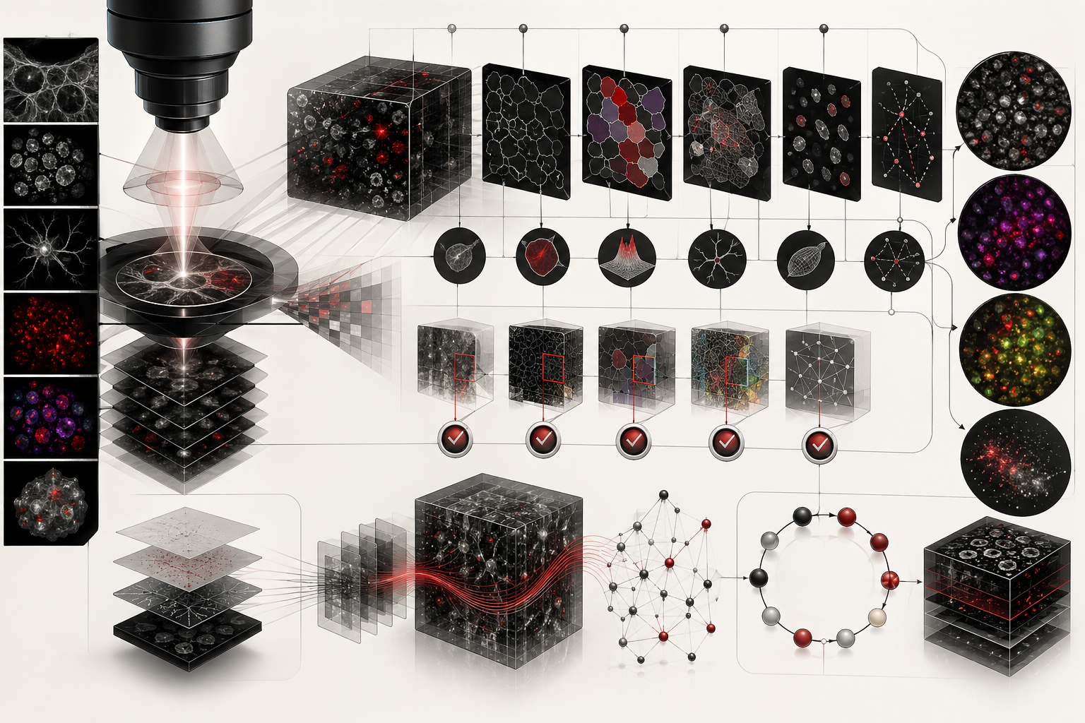
The article is written for biologists, cell biologists, developmental biologists, neuroscientists, microbiologists, biomedical researchers, computational biologists, bioimage analysts, laboratory scientists, data engineers, scientific software developers, imaging-core teams, and engineers. It emphasizes image formation, metadata, segmentation, feature extraction, registration, tracking, colocalization, high-content screening, reproducibility, provenance, quality control, and responsible computational interpretation.

The article also extends the discussion into reproducible computational practice through Python and R examples, synthetic microscopy arrays, threshold segmentation, object labeling, intensity-feature extraction, colocalization scaffolds, tracking summaries, SQL-backed provenance, validation metrics, and a linked full-stack GitHub repository containing Python, R, Julia, Fortran, Rust, Go, C, C++, SQL, notebooks, data files, validation notes, and reproducibility documentation.

Why Microscopy Image Analysis Matters

Microscopy image analysis matters because much of biology is spatial, visual, and dynamic. Cells change shape. Organelles move. Tissues pattern. Microbes grow. Neurons branch. Embryos develop. Proteins localize. Immune cells migrate. Tumors invade. Plant tissues organize. Biofilms form. These processes cannot be fully understood from tables alone because location, morphology, intensity, adjacency, and movement are biologically meaningful.

Manual visual inspection remains indispensable for discovery, quality control, and expert interpretation, but it is difficult to scale and can vary across observers. Computational analysis makes image-based evidence explicit by producing masks, object tables, trajectories, spatial graphs, intensity summaries, uncertainty estimates, and reviewable failure cases. The aim is not to automate away expertise. It is to connect expertise to measurements that can be audited and repeated.

Modern microscopy also produces data at scales that exceed unaided inspection. A single experiment may contain hundreds of wells, thousands of fields, millions of cells, multiple channels, z-stacks, time points, treatment conditions, and imaging batches. The scientific challenge is therefore not only seeing structures. It is building a measurement system that remains reliable from specimen preparation through acquisition, computation, statistics, and interpretation.

Computational microscopy helps scientists ask three linked questions: what was observed, how was it transformed into a measurement, and how much confidence should be placed in the resulting biological claim?

Images as Biological Measurements

A microscopy image is not a direct copy of biological reality. It is the output of a measurement chain involving a specimen, contrast mechanism, optical system, illumination source, detector, acquisition settings, digitization process, and computational pipeline. Every link can change the values that appear in the image.

In fluorescence microscopy, measured intensity can depend on labeling specificity, fluorophore maturation, concentration, quantum yield, illumination power, exposure time, bleaching, detector gain, read noise, background, autofluorescence, spectral bleed-through, optical blur, and sample thickness. In brightfield and histology, staining, section thickness, illumination, focus, scanner response, tissue folding, compression, and color normalization shape the image. Electron and super-resolution microscopy introduce different preparation, reconstruction, and resolution assumptions.

The same biological specimen can therefore yield different images under different systems. Quantitative comparison requires either consistent acquisition or a justified calibration and normalization strategy. An intensity difference cannot automatically be interpreted as a molecular abundance difference. A boundary cannot be treated as exact when the point-spread function and sampling grid blur the underlying structure.

Images become scientific evidence when the biological quantity of interest, acquisition process, image representation, analysis algorithm, and inferential claim are connected in one traceable workflow.

The Imaging Measurement Chain and Fitness for Purpose

Reliable bioimage analysis begins by defining the measurand: the quantity intended to be measured. The measurand might be nuclear count per field, cell area in square micrometers, integrated fluorescence per object, organelle number, migration speed, vessel length density, marker-positive fraction, neighborhood enrichment, or a treatment-induced morphological profile. Each requires a different level of image quality and analysis performance.

Fitness for purpose is more useful than asking whether an image or algorithm is simply “good.” A segmentation with modest boundary agreement may be adequate for counting well-separated nuclei but inadequate for measuring membrane thickness. A low-magnification scan may support tissue-area estimation but not subcellular localization. A denoised image may be suitable for visualization yet inappropriate for intensity quantification if the transformation changes photon statistics.

Biological claim	Minimum measurement need	Common failure
Count nuclei	Reliable object separation and field coverage	Under-segmentation in crowded regions
Compare fluorescence abundance	Unsaturated acquisition, background control, stable detector response	Gain or illumination differences interpreted as biology
Measure migration	Stable registration, sufficient frame rate, validated linking	Drift or track swapping treated as movement
Measure colocalization	Channel registration, bleed-through control, justified spatial statistic	Optical blur interpreted as molecular interaction
Profile treatment phenotypes	Randomized plates, controls, batch correction, independent units	Plate position or confluence driving the profile

A defensible project states the intended claim before acquisition and derives quality-control thresholds, annotation plans, validation metrics, and statistical units from that claim.

Pixels, Voxels, Channels, and Metadata

Microscopy data are commonly multidimensional. A dataset may include two or three spatial dimensions, multiple channels, time, fields, wells, tiles, positions, samples, and experimental conditions. A pixel records a detector-derived value on a two-dimensional grid. A voxel extends that representation into three dimensions. Neither is a biological object by itself.

Spatial calibration converts pixel or voxel indices into physical coordinates. Pixel size, z-spacing, stage position, objective magnification, numerical aperture, refractive index, and image orientation influence interpretation. An object area reported only in pixels cannot be compared safely across magnifications. A z-stack with coarse axial sampling may not support reliable volume or surface measurements.

Metadata are part of the measurement. Channel identity, excitation and emission ranges, exposure, illumination power, detector mode, gain, binning, objective, numerical aperture, immersion medium, acquisition time, sample identifier, plate position, and processing history all affect the meaning of the numbers. Dimensional axes should be explicit rather than inferred from filename conventions.

OME-XML and related OME data models provide structured representations for pixels, acquisition settings, regions of interest, and experimental annotations. OME-NGFF extends this direction toward chunked, cloud-compatible multidimensional bioimaging data. In August 2026, OME-NGFF 0.5 is the latest published version, while 0.6 remains a release-candidate or development line; production workflows should distinguish stable specifications from editor drafts.

Optics, the Point-Spread Function, and Sampling

Microscopes do not reproduce point objects as perfect points. The optical system spreads signal according to a point-spread function. Resolution is therefore not identical to pixel size, and increasing digital magnification cannot recover information that the optics and sampling did not capture.

Objective numerical aperture, wavelength, refractive-index matching, aberrations, alignment, pinhole settings, detector sampling, and specimen depth all influence effective resolution. Axial resolution is usually poorer than lateral resolution, which makes three-dimensional objects anisotropic in the raw image. Chromatic aberration can shift channels relative to one another and create false spatial conclusions.

Nyquist sampling provides a practical principle: sample finely enough to represent the spatial information passed by the optical system. Undersampling loses detail and destabilizes segmentation. Oversampling can enlarge files and increase exposure without adding equivalent biological information. The correct balance depends on the measurement goal.

\[
d \approx \frac{0.61\lambda}{NA}
\]

Interpretation: A simplified lateral-resolution expression relates resolvable distance \(d\) to wavelength \(\lambda\) and numerical aperture \(NA\). Real performance also depends on alignment, aberration, contrast, sampling, and specimen conditions.

Point-spread-function measurements with suitable reference objects can reveal changes in lateral resolution, axial resolution, symmetry, and alignment. They are instrument quality-control measurements, not only theoretical optics.

Instrument Calibration and Longitudinal Quality Control

Quantitative microscopy depends on an instrument that is characterized over time. Illumination power and stability, detector conversion, read noise, dynamic range, stage precision, channel registration, field uniformity, and point-spread function can drift. Without longitudinal quality control, a biological trend can be confounded with an instrument trend.

QUAREP-LiMi organizes community work around practical quality assessment and reproducibility for light microscopy, including illumination, detector performance, co-registration, resolution, metadata, and publication standards. Its 2026 materials emphasize photon characterization, point-spread-function monitoring, co-registration, and the Light-Microscopy Metadata Model. These efforts move microscopy from informal visual checks toward documented measurement assurance.

A quality-control program should define reference samples, acquisition procedures, metrics, acceptable limits, frequency, corrective actions, and the relationship between QC results and experimental data. Reference images should be stored with dates, configuration identifiers, software versions, and instrument maintenance records.

Calibration cannot make every experiment comparable automatically. Reference materials may not mimic the biological specimen, and a stable instrument does not correct inconsistent staining or sample preparation. Calibration should be treated as one layer in a larger uncertainty budget.

Image Quality, Dynamic Range, and Noise

Image quality determines which claims are supportable. Saturation destroys intensity ranking. Low signal-to-noise ratio destabilizes detection and segmentation. Uneven illumination creates artificial spatial gradients. Background and autofluorescence reduce contrast. Focus variation changes texture and apparent object size. Compression and resampling can damage quantitative relationships.

Noise is not a single phenomenon. Photon shot noise, detector read noise, dark current, fixed-pattern noise, digitization, reconstruction artifacts, and biological background have different behavior. A denoising method that assumes additive Gaussian noise may be poorly matched to photon-limited imaging. Quality metrics should therefore reflect the acquisition process.

Useful checks include saturation fraction, background mean and variance, signal-to-background ratio, focus score, illumination uniformity, object count, intensity distribution, and channel correlation. These checks should be examined by plate, batch, field, sample, and time, not only globally.

Quality-control exclusion must also be pre-specified and documented. Removing images because they weaken an expected result creates bias. Exclusion should be tied to measurement failure, not biological outcome.

Quantitative Fluorescence and Photon-Aware Analysis

Fluorescence intensity is often treated as a direct proxy for molecular abundance, but digital intensity values are produced by a detector and acquisition configuration. Camera offset, conversion gain, quantum efficiency, exposure, illumination, bit depth, and nonlinear processing determine how photons become pixel values.

Photon-transfer characterization can estimate detector gain, read noise, and dynamic range. Flat-field and dark-reference measurements can reveal nonuniform illumination and offset. These measurements help distinguish arbitrary digital units from physically interpretable or at least comparable detector response.

Quantitative fluorescence also depends on the specimen. Labeling stoichiometry, fluorophore maturation, quenching, environmental sensitivity, bleaching, fixation, and accessibility can change intensity independently of target abundance. Absolute quantification may require calibrated reference materials or fluorescence standards; relative quantification still requires acquisition within a validated linear range.

Ratio images and normalized intensities do not automatically remove bias. Noise and background propagate through ratios, and normalization to a changing reference can create artifacts. Photon-aware analysis should preserve unsaturated raw counts, characterize background, and report how conversion and correction were performed.

Specimen Preparation, Labeling, and Biological Artifacts

Image analysis begins with biology and specimen preparation. Fixation can shrink, swell, crosslink, extract, or redistribute structures. Permeabilization changes membranes. Clearing changes refractive properties. Sectioning can truncate objects. Stains differ in specificity, penetration, dynamic range, and batch stability. Live imaging introduces phototoxicity, environmental stress, and temporal constraints.

Labeling controls are essential. Negative controls help estimate background and nonspecific binding. Single-label controls help characterize bleed-through. Positive controls test whether the assay can detect the intended signal. Isotype or secondary-only controls may be useful in immunofluorescence, depending on assay design. Genetic or orthogonal validation can strengthen interpretation.

Artifacts can be biologically structured. Tissue folds, bubbles, debris, dead cells, autofluorescent regions, edge effects, and density gradients may cluster by sample or treatment. An algorithm may learn these artifacts and still achieve high apparent accuracy.

A robust workflow records specimen age, preparation protocol, reagent lots, fixation time, staining batch, handling delays, environmental conditions, and deviations. These variables belong in the provenance chain and may need explicit modeling.

Preprocessing, Restoration, and Deconvolution

Preprocessing may include flat-field correction, background subtraction, denoising, deconvolution, registration, color normalization, resampling, or illumination correction. Each transformation changes the data and should be justified by the measurement objective.

Deconvolution estimates a sharper underlying object from blurred measurements using a point-spread-function model and assumptions about noise. It can improve contrast and separation, but it does not create certainty. Results depend on the PSF, boundary conditions, iteration count, regularization, and mismatch between model and specimen.

Preprocessing order matters. Background subtraction before ratio calculation may behave differently from subtraction afterward. Resampling masks can change object area. Normalizing each image independently can erase meaningful global intensity differences. Using information from test data to choose preprocessing can leak outcome information into validation.

Raw data should be preserved. Processed derivatives should be linked to raw inputs through explicit parameters, software versions, and checksums. Visualization-oriented transformations should be clearly separated from quantitative inputs.

Segmentation and Object Detection

Segmentation assigns pixels or voxels to objects, regions, or background. Object detection estimates locations or bounding regions without necessarily defining every boundary. In microscopy, targets include nuclei, whole cells, membranes, organelles, vessels, colonies, plaques, lesions, fibers, synapses, microbes, and tissue compartments.

Classical methods include thresholding, watershed, edge detection, morphology, region growing, active contours, graph cuts, and model-based fitting. Machine-learning and deep-learning systems can learn more complex appearance patterns. The appropriate method depends on contrast, object topology, density, dimensionality, annotation availability, and intended measurement.

Segmentation is not merely a preprocessing step. It defines the units from which counts, areas, intensities, textures, neighborhoods, and trajectories are calculated. Merged cells reduce counts and inflate areas. Split nuclei increase counts. Boundary bias changes membrane and cytoplasmic intensity. Missed faint objects can create group-specific undercounting.

Algorithms should preserve uncertainty where possible. Borderline pixels, ambiguous touching objects, and low-confidence detections can be flagged for review rather than forced into false certainty.

Ground Truth, Annotation, and Segmentation Validation

Segmentation validation requires reference information, but “ground truth” is often an approximation produced by experts under the same resolution limits as the image. Annotators may disagree about faint boundaries, overlapping cells, fragmented objects, or biological definitions. Annotation protocols should therefore define inclusion rules, object identity, edge cases, and adjudication.

Validation should match the biological use. Pixel overlap metrics such as Dice and Intersection over Union assess mask agreement. Object-level precision and recall assess detection. Split and merge errors assess topology. Boundary distances assess contour accuracy. Count bias, area bias, and intensity bias assess downstream measurement consequences.

\[
Dice=\frac{2|A\cap B|}{|A|+|B|}
\]

Interpretation: Dice summarizes overlap between predicted mask \(A\) and reference mask \(B\). A high Dice score does not guarantee correct object separation or unbiased biological measurements.

Validation data should be independent of model fitting and parameter tuning. It should cover multiple batches, specimens, instruments, and difficult cases. Reporting only a mean score can conceal catastrophic failures in rare but important image types.

Uncertainty from Pixels to Biological Estimates

Image-derived uncertainty accumulates across acquisition, preprocessing, segmentation, feature extraction, sampling, and statistical modeling. A single confidence score from a neural network does not represent this full chain.

Threshold sensitivity, alternative segmentations, annotation disagreement, replicate acquisitions, bootstrap resampling, and simulation can reveal how results change under plausible analysis choices. For example, a treatment effect that disappears under a small threshold change is less robust than one that persists across validated parameter ranges.

Uncertainty should be reported at the level of the biological claim. If cells are nested within fields, fields within wells, and wells within biological samples, thousands of segmented cells do not create thousands of independent experimental units. The uncertainty of a treatment effect depends on independent samples, batch structure, measurement error, and model assumptions.

Where algorithmic uncertainty is difficult to calibrate, transparent sensitivity analysis is preferable to an unjustified probability. The goal is not to assign a precise number to every unknown. It is to show which conclusions are stable and which depend on fragile decisions.

Feature Extraction and Biological Phenotypes

Image features summarize object morphology, intensity, texture, topology, spatial position, and context. Common features include count, area, perimeter, eccentricity, solidity, intensity mean, integrated intensity, granularity, spot number, skeleton length, branching, radial distribution, nearest-neighbor distance, and neighborhood composition.

Features are measurements, not automatically phenotypes. Nuclear size may relate to cell cycle, senescence, ploidy, or segmentation bias. Mitochondrial texture may reflect morphology, focus, staining, or illumination. Marker intensity may approximate abundance only within a validated response range.

Feature definitions should specify units, masks, channels, background correction, aggregation, and handling of missing or saturated values. High-dimensional projects should control redundancy and prevent feature selection from using information from held-out samples.

Biological interpretation is strengthened when image-derived features are linked to orthogonal evidence such as flow cytometry, biochemical assays, genetics, clinical variables, or independent imaging modalities.

Morphology, Texture, and Shape Representation

Shape and texture encode biological organization beyond simple size. Circularity, elongation, convexity, curvature, skeletons, fractal descriptors, radial profiles, co-occurrence matrices, local binary patterns, multiscale filters, and learned embeddings can distinguish cellular and tissue states.

These representations are sensitive to scale and orientation. A texture feature calculated at one pixel spacing may not be comparable after resampling. Two-dimensional shape may misrepresent a three-dimensional object. Rotationally invariant descriptors may remove biologically meaningful orientation.

Learned image embeddings can capture complex phenotypes without hand-crafted feature definitions, but their dimensions may be difficult to interpret. Embeddings should be evaluated for batch sensitivity, stability, nearest-neighbor coherence, treatment recovery, and transfer across datasets.

A good representation is not simply the one that maximizes classification accuracy. It should preserve the biological differences relevant to the question while minimizing irrelevant acquisition variation.

Registration, Colocalization, and Spatial Structure

Registration aligns images across channels, time points, tiles, z-planes, or modalities. Drift correction supports time-lapse analysis; chromatic registration supports multichannel localization; tissue registration supports longitudinal and multimodal comparison. Registration transforms should be stored and validated.

Colocalization can refer to intensity correlation, fractional overlap, object proximity, or enrichment relative to a spatial null model. These are different questions. Pearson correlation can be influenced by background and intensity gradients. Manders-type coefficients depend on thresholds. Object-based distances require reliable segmentation. Dense structures and optical blur can create apparent overlap without molecular interaction.

Spatial analysis extends beyond colocalization. Cell neighborhoods, tissue compartments, immune infiltration, distances to vessels, point-pattern clustering, boundary enrichment, and spatial graphs can reveal organization that is invisible in global averages.

Appropriate null models matter. Randomizing points across an impossible tissue region produces misleading significance. Spatial tests should preserve relevant geometry, density, masks, and sampling constraints.

Three-Dimensional Imaging and Volume Analysis

Confocal, light-sheet, cleared-tissue, tomography, and electron-microscopy workflows increasingly produce volumetric data. Three-dimensional analysis can measure volume, surface area, branching, connectivity, contact, distance, and organization that two-dimensional sections cannot represent faithfully.

Volumes are often anisotropic: z-spacing and axial resolution differ from lateral sampling. Algorithms should use physical spacing when calculating distances, surfaces, and morphology. Resampling to isotropic voxels may simplify computation but changes interpolation and memory requirements.

Large volumes create practical challenges in storage, chunking, visualization, annotation, and distributed computation. Multiscale representations allow rapid viewing while retaining access to full-resolution data. OME-NGFF and chunked Zarr-based approaches address this need for cloud-compatible bioimaging.

Validation should include structures of different sizes, depths, and orientations. A model that performs well near the coverslip may fail deep in tissue because of scattering, attenuation, and aberration.

Spatial Omics, Tissue Atlases, and Multimodal Registration

Spatial transcriptomics, multiplexed imaging, imaging mass cytometry, cyclic immunofluorescence, and tissue-atlas projects combine morphology with molecular identity. Their central challenge is coordinate integration: cells, spots, molecules, tissue regions, and anatomical structures must be mapped into a shared spatial frame.

Segmentation errors can propagate into cell-by-feature matrices. A boundary that assigns transcripts or proteins to the wrong cell changes apparent cell state and neighborhood relationships. Spot-based assays introduce partial-volume effects because one measurement region may contain multiple cells. Registration between histology and molecular channels can distort local geometry.

Multimodal analysis should preserve the distinction between measured and inferred resolution. Computational deconvolution of spots into cell types does not create single-cell measurement certainty. Tissue compartments and cell neighborhoods should be validated against morphology and independent markers.

Atlas-scale projects also require coordinate systems, ontologies, multiscale storage, sample provenance, and cross-donor modeling. A reference atlas is not a universal normal state; population, developmental, disease, and preparation differences remain biologically important.

Tracking, Time-Lapse, and Dynamic Biology

Time-lapse microscopy converts biological change into sequences. Tracking links detections across frames to estimate displacement, speed, persistence, lineage, division, death, interaction, and state transition. The analysis depends on detection quality, frame interval, motion model, and treatment of gaps.

Track errors include identity swaps, fragmentation, false continuation, missed division, and incorrect parent-child assignment. A small number of errors can strongly bias lineage duration, migration persistence, and interaction timing. Validation should include event-level metrics, not only average localization error.

Imaging frequency creates trade-offs. Long intervals miss fast events and create ambiguous links. Short intervals increase light exposure, storage, and phototoxicity. The acquisition plan should match the dynamic scale of the biological process.

Stage drift, focus changes, changing illumination, bleaching, and cell-density growth create time-dependent confounding. These should be monitored alongside trajectories.

Lineage Reconstruction, Event Detection, and State Transitions

Dynamic analysis often requires identifying discrete events: mitosis, apoptosis, differentiation, fusion, entry into a region, signaling pulses, organelle fission, or phenotype transition. Event definitions should be biological and operational. A model must know what temporal evidence qualifies as an event.

Lineage trees connect cells across generations and can reveal heritable state, treatment response, and developmental dynamics. They are especially sensitive to missing frames and identity errors. Manual correction interfaces and confidence flags can be more valuable than fully automatic but opaque output.

State transitions can be modeled from image features, reporter intensities, morphology, or learned embeddings. Hidden-state models may distinguish noisy observations from latent biological states, but states should not be interpreted mechanistically without perturbation or orthogonal evidence.

Temporal conclusions require independent biological replication. Thousands of frames from one dish remain one experimental context.

High-Content Screening and Image-Based Profiling

High-content screening combines automated microscopy with large perturbation spaces: compounds, genes, doses, cell lines, organoids, and time points. Image-based profiling converts cellular appearance into multivariate signatures that can group mechanisms, identify outliers, and support phenotypic discovery.

Experimental design is inseparable from analysis. Controls should be distributed across plates. Treatments should be randomized or blocked. Edge wells, confluence, dispensing, staining, and imaging order should be monitored. Plate-level normalization should not erase true global responses.

Profiles may be aggregated from cells to wells and from wells to biological replicates. The aggregation rule affects sensitivity to subpopulations. Median profiles are robust but may hide rare responders. Distributional or mixture approaches can preserve heterogeneity.

Evaluation can include replicate consistency, control separation, known mechanism recovery, cross-batch reproducibility, and performance on unseen plates. A profile useful for retrieval is not automatically a causal explanation.

Batch Effects and Experimental Design

Microscopy experiments are vulnerable to plate, day, operator, reagent, microscope, objective, sample, and processing batches. Because image-derived data are high dimensional, batch differences can dominate biological differences while remaining visually subtle.

Randomization distributes nuisance variation across conditions. Blocking places relevant comparisons within manageable acquisition or preparation groups. Controls estimate technical structure. Replication across days or instruments tests transportability. These design decisions are more reliable than trying to remove every problem computationally afterward.

Batch correction should be evaluated against negative and positive controls and should preserve known biology. Overcorrection can remove treatment effects. Under-correction can leave technical clusters. Correction parameters must be learned without leaking held-out outcomes.

The independent unit must be explicit. Cells nested within one well do not replace independent wells; wells from one culture do not replace independent cultures; sections from one patient do not replace patients.

Deep Learning and Bioimage Analysis

Deep learning has expanded segmentation, detection, classification, restoration, super-resolution, tracking, and representation learning. These models can learn complex appearance patterns and reduce manual parameter engineering, but their performance depends on data provenance and deployment context.

Training data should document specimens, microscopes, channels, labels, annotation procedures, preprocessing, splits, and exclusions. Random image-level splitting can leak nearly identical fields or cells from the same specimen into training and test sets. Splits should respect the intended generalization unit.

Model validation should include calibration, failure modes, subgroup performance, external batches, and biologically meaningful downstream metrics. High average accuracy can conceal poor performance on rare phenotypes, low-signal images, or underrepresented tissues.

Deep learning is most useful when embedded in a reviewable pipeline with versioned models, known input requirements, confidence handling, and a route for expert correction.

Pretrained Models, Foundation Models, and the BioImage Model Zoo

Pretrained bioimage models can reduce annotation burden and make advanced analysis available to more laboratories. The BioImage Model Zoo provides a community platform for discovering and deploying interoperable models, while tools such as napari, Fiji, CellProfiler, and Python libraries provide interfaces for integration and review.

Model reuse requires more than downloading weights. The input axes, channel semantics, pixel size, normalization, expected intensity range, output classes, license, training domain, and software dependencies must be compatible. A nucleus model trained on one stain and resolution may fail silently on another.

Foundation-style models aim to support broad transfer across imaging tasks, but broad pretraining does not remove the need for local validation. Generalization claims should be tested across specimens, labs, instruments, and populations relevant to use.

Reusable models should be treated as scientific artifacts with identifiers, version history, documentation, evaluation data, and provenance, not as undocumented plugins.

Restoration, Denoising, and Hallucination Risk

Computational restoration can improve visibility under low-light or fast acquisition, but it creates a special inferential risk: a visually convincing result may contain structures not sufficiently supported by the measurement. Neural denoising and super-resolution models learn priors from training data and may reproduce expected patterns when evidence is weak.

Restored images should be compared with raw data and suitable references. Quantitative measurements should be validated for bias after restoration. Split-image or self-supervised methods reduce some data requirements but do not guarantee biological fidelity.

Uncertainty maps, residual analysis, frequency-domain checks, simulated structures, and blinded expert review can help reveal failure. For high-consequence claims, orthogonal imaging or perturbation evidence may be necessary.

Figures should disclose restoration methods and avoid presenting generated detail as direct observation. Raw data should remain accessible.

Domain Shift, Generalization, and Model Monitoring

Domain shift occurs when deployment images differ from training data. Differences may arise from species, tissue, disease state, microscope, objective, detector, stain, lot, resolution, background, compression, or laboratory practice. A model can fail even when images look similar to a human observer.

External validation should reflect actual deployment conditions. Performance should be stratified by relevant groups and image-quality ranges. Out-of-distribution detection may help identify unfamiliar inputs, but such detectors also require validation.

Model monitoring is needed when instruments, protocols, and populations change over time. Input summaries, segmentation distributions, confidence patterns, QC failures, and manually reviewed samples can indicate drift. Revalidation should follow meaningful workflow changes.

Versioning should connect every result to the exact model, code, parameters, and environment used. Silent model replacement breaks reproducibility.

Benchmarking, Challenge Datasets, and Task Definition

Benchmarking helps compare methods, but benchmark results are only meaningful when the task, reference annotations, data splits, and evaluation metrics match the intended use. A leaderboard can reward narrow optimization while overlooking biological validity and external generalization.

Datasets should separate training, validation, and test specimens at the correct hierarchy. Holding out random tiles from the same tissue slide does not test slide-level generalization. Hidden test labels reduce tuning, while external-site datasets test transportability more directly.

Multiple metrics are usually needed. Detection precision and recall, instance segmentation quality, boundary accuracy, split and merge rates, tracking association, calibration, inference time, memory, and downstream measurement bias represent different properties. Ranking methods by one aggregate score can hide important trade-offs.

Challenge datasets should document licensing, consent, annotation uncertainty, class prevalence, acquisition diversity, and known artifacts. A benchmark is a measurement system for algorithms and requires the same scrutiny as the algorithms it evaluates.

Human-in-the-Loop Analysis, Annotation, and Active Learning

Expert review is often most valuable when directed toward ambiguous and consequential cases. Human-in-the-loop workflows allow analysts to correct masks, review low-confidence objects, adjudicate rare phenotypes, and refine model behavior.

Active learning can prioritize examples expected to improve a model, but selection should not focus only on algorithmic uncertainty. Rare biological classes, important subgroups, and known artifact types may need deliberate inclusion.

Annotation interfaces should preserve original context, scale, channels, and neighboring structures. Annotator identity, training, protocol version, and correction history should be recorded. Agreement statistics can reveal unclear definitions.

Human correction is not automatically ground truth. Reviewers can share biases and may be influenced by model suggestions. Blinded review, independent annotation, and periodic quality checks can reduce anchoring.

Statistics, Units of Analysis, and Image-Derived Data

Image analysis often creates many rows from few independent samples. Cells are nested within fields, fields within wells, wells within plates, sections within specimens, and specimens within organisms or patients. Statistical models should represent this hierarchy.

Pseudoreplication occurs when segmented objects are treated as independent biological replicates. It can produce extremely small p-values while the actual experiment has weak replication. Mixed-effects models, cluster summaries, hierarchical bootstrap methods, and specimen-level analyses can respect the design.

Feature distributions may be skewed, zero-inflated, bounded, censored, or multimodal. Outlier removal should distinguish artifacts from legitimate biological extremes. Multiple-testing control is needed when hundreds or thousands of features are screened.

Effect sizes and uncertainty intervals are usually more informative than significance alone. The analysis should report the magnitude of biological change and its stability across independent units and analysis choices.

Image Data Standards: OME-TIFF, OME-XML, and OME-NGFF

Bioimage data are difficult to reuse when pixels, axes, and acquisition metadata are trapped in proprietary formats. Bio-Formats translates many vendor formats into OME-compatible representations. OME-XML describes multidimensional pixels and extensive acquisition metadata. OME-TIFF embeds OME-XML with TIFF pixel data for broad compatibility.

OME-NGFF addresses large, chunked, multiscale, cloud-compatible data. Version 0.5 is the latest published specification in August 2026, and it uses Zarr version 3. Development work toward 0.6 includes richer coordinate systems and transformations. Workflows should pin the specification version rather than referring generically to “OME-Zarr.”

Standards do not guarantee complete metadata. Export tools may lose vendor-specific details, and conversions should be checked. The data model must also be supplemented with biological and experimental context.

Interoperability is strongest when files, metadata, derived labels, tables, coordinate transforms, and provenance are designed together.

Open-Source Tools and Pipeline Interoperability

Bioimage analysis is supported by a broad open-source ecosystem. Fiji and ImageJ provide interactive processing and macros. CellProfiler provides modular pipelines for quantitative high-throughput analysis. napari supports multidimensional visualization, annotation, and plugins. scikit-image and related Python libraries support programmable processing. OMERO supports image management, visualization, and collaborative access.

Interoperability should not be assumed. Tools may differ in axis order, coordinate conventions, label representation, interpolation, metadata handling, and file-writing behavior. Converting data or masks between tools requires validation of dimensions, physical scale, channel identity, and object labels.

Pipeline design can combine interactive and scripted components. Experts may annotate in napari, manage data in OMERO, analyze images in CellProfiler or Python, and archive outputs in OME-compatible formats. The reproducibility requirement is that each handoff be explicit and testable.

Plugins and dependencies should be pinned by version. A graphical workflow is not inherently irreproducible, and code is not inherently reproducible; both depend on captured state, stable inputs, and verifiable outputs.

FAIR Image Data, REMBI, and Public Archives

FAIR bioimage data should be findable, accessible, interoperable, and reusable. Reuse requires more than uploading a large file. Researchers need sample context, acquisition metadata, image organization, analysis outputs, and rights information.

The BioImage Archive is EMBL-EBI’s broad, cross-modality resource for biological images and implements Recommended Metadata for Biological Images guidance. It archives data associated with publications or valuable beyond a single experiment and supports downstream resources such as EMPIAR and the evolving Cell-IDR and Tissue-IDR ecosystem. It does not accept patient-identifiable medical images.

QUAREP-LiMi’s metadata work, including the Light-Microscopy Metadata Model, aims to harmonize hardware, acquisition, and quality-control description and to support FAIR-by-design workflows. Its publication-standards work also promotes minimal microscopy methods reporting and raw-data availability.

Data release should consider consent, privacy, licensing, embargo, file integrity, and whether derived masks, annotations, models, and analysis code are included alongside raw images.

Workflow Provenance and Reproducible Computation

Provenance connects each result to its inputs and transformations. A reproducible microscopy project should identify raw files, checksums, sample metadata, acquisition settings, preprocessing operations, segmentation model or parameters, feature definitions, exclusions, aggregation, statistical code, and output versions.

Interactive tools can be reproducible when their settings and actions are exportable. CellProfiler pipelines, Fiji macros, napari plugins, notebooks, command-line workflows, containers, and workflow engines can all support reproducibility if versions and parameters are captured.

Random seeds, hardware libraries, model weights, dependency locks, and environment information matter for machine learning and stochastic analysis. Large data may require object storage and chunked access; the workflow should still preserve immutable source references.

Reproducibility should be tested by rebuilding outputs from a clean environment. A manuscript methods paragraph is not a substitute for an executable record.

Figure Preparation and Microscopy Methods Reporting

Published figures are scientific interfaces, not decorative summaries. Scale bars should be derived from spatial calibration rather than typed manually. Channel colors, lookup tables, contrast ranges, projections, crops, and annotations should be described. Comparisons should use consistent display transformations unless a difference is clearly justified.

Microscopy methods should report specimen preparation, modality, objective, numerical aperture, immersion medium, detector, pixel size, z-step, channels, exposure, illumination, acquisition software, preprocessing, segmentation, validation, and statistical units relevant to the claim. “Images were analyzed in ImageJ” is not sufficient.

QUAREP-LiMi’s publication-standards work has promoted bare-minimum reporting requirements aligned with REMBI and microscopy metadata models. These efforts recognize that reproducibility depends on coordinated expectations from researchers, imaging scientists, reviewers, journals, and funders.

Representative images should be paired with quantitative summaries from the full sampling design. Raw or minimally processed data, analysis masks, and methods should be available for validation when governance permits.

Environmental and Ecological Microscopy

Computational microscopy also applies beyond cells and tissues in controlled laboratories. Plankton imaging, microbial ecology, sediment microscopy, soil microstructure, environmental particles, coral histology, plant anatomy, and automated taxonomic imaging connect microscopic observations to ecological monitoring.

Environmental samples are heterogeneous and often contain debris, mixed organisms, variable preservation, and strong seasonal or geographic structure. Training data from one water body or sampling device may not transfer to another. Taxonomic uncertainty and open-set recognition are central because unknown or rare organisms may appear.

Sampling design must connect image counts to sampled volume, area, flow, depth, or effort. An automated classifier can count objects accurately while the ecological abundance estimate remains biased by collection and detection. Calibration of the imaging instrument does not replace calibration of the field-sampling process.

Ecological image archives and reference collections can support reuse, but they should preserve specimen provenance, geographic sensitivity, taxonomic authority, and environmental metadata.

Ethics, Privacy, and Responsible Image Analysis

Biomedical images can contain patient-derived tissue, clinical context, rare-disease information, facial or anatomical identifiers, and metadata that enable re-identification. Consent and data-governance requirements depend on the specimen, jurisdiction, repository, and intended reuse.

Algorithmic performance may differ across tissues, demographics, disease states, and laboratories. Biased annotations or unrepresentative data can produce unequal error. These issues matter even in preclinical research because image-derived models may shape downstream targets, biomarkers, and clinical tools.

Manipulation and presentation also carry ethical obligations. Contrast changes, channel selection, cropping, restoration, and representative-image choice should not distort interpretation. Quantitative conclusions should not rely on a single aesthetically selected field.

Responsible image analysis preserves raw data, documents transformations, communicates uncertainty, protects sensitive information, and maintains human accountability for biological claims.

Mathematical Lens: Image Analysis and Uncertainty

Mathematical notation helps separate image formation, segmentation, validation, and downstream inference. The equations below are simplified representations whose usefulness depends on calibration and model assumptions.

Image formation

\[
I_{obs}=H*I_{true}+\epsilon
\]

Interpretation: The observed image is represented as the underlying object convolved with optical response \(H\), plus noise and unmodeled effects \(\epsilon\).

Threshold segmentation

\[
M(x,y)=\begin{cases}1 & I(x,y)\ge\tau\\0 & I(x,y)<\tau\end{cases}
\]

Interpretation: Threshold \( au\) defines a binary mask. Sensitivity to \( au\) is a basic uncertainty test.

Signal-to-noise ratio

\[
SNR=\frac{\mu_s-\mu_b}{\sigma_b}
\]

Interpretation: Signal separation from background variability affects detection and measurement reliability.

Intersection over Union

\[
IoU=\frac{|A\cap B|}{|A\cup B|}
\]

Interpretation: IoU measures mask overlap but does not independently measure object topology or downstream feature bias.

Object centroid

\[
\bar{x}=\frac{1}{n}\sum_i x_i,\qquad \bar{y}=\frac{1}{n}\sum_i y_i
\]

Interpretation: Centroids support tracking and spatial analysis when masks are valid.

Pearson channel correlation

\[
r=\frac{\sum_i(X_i-\bar{X})(Y_i-\bar{Y})}{\sqrt{\sum_i(X_i-\bar{X})^2}\sqrt{\sum_i(Y_i-\bar{Y})^2}}
\]

Interpretation: Intensity correlation is affected by background, gradients, bleed-through, and spatial resolution.

Tracking displacement

\[
d_t=\sqrt{(x_{t+1}-x_t)^2+(y_{t+1}-y_t)^2}
\]

Interpretation: Frame-to-frame displacement is a geometric measurement; biological motion interpretation also requires drift correction and validated identity linking.

Hierarchical measurement model

\[
y_{ijk}=\mu+\alpha_i+b_{ij}+\epsilon_{ijk}
\]

Interpretation: Observations \(k\) are nested within fields or wells \(j\) and biological units \(i\), separating treatment, sample, and image-level variation.

Threshold sensitivity

\[
S_\tau=\frac{\Delta g}{\Delta \tau}
\]

Interpretation: Sensitivity of biological estimate \(g\) to threshold changes reveals parameter fragility.

Worked Diagnostic: A Multibatch Live-Cell Imaging System

Consider a study measuring treatment-induced changes in cell migration and nuclear morphology across three biological experiments, two microscopes, four plates per experiment, and six fields per well. The workflow uses fluorescence nuclei, phase-contrast cell bodies, automated segmentation, and time-lapse tracking. The purpose is to determine whether an apparent treatment response is biological or produced by image quality, batch structure, segmentation, or tracking failure.

Step 1: Define the claim and independent unit

The primary claim is a change in specimen-level median migration speed. Independent biological experiments, not cells or frames, are the primary replication units. Nuclear area and track persistence are secondary measurements.

Step 2: Inspect acquisition quality

One microscope shows a gradual focus decline late in acquisition, and two plates contain illumination gradients. Saturation is low, but background rises over time. These findings are mapped to wells and frames rather than summarized only at dataset level.

Step 3: Validate channel registration and drift correction

Bead controls show acceptable registration on one microscope and a systematic channel offset on the second. Stage landmarks reveal slow drift. Registration and drift transforms are estimated from controls and stored with provenance.

Step 4: Evaluate segmentation by biological use

Dice overlap is high for nuclei, but crowded fields show merge errors that bias counts and area. Object-level split and merge rates are therefore examined alongside overlap. Crowded fields are flagged rather than silently accepted.

Step 5: Evaluate tracking and event logic

Track identity swaps increase when cells cross. A reviewed subset shows that speed is less biased than lineage duration, while persistence is moderately sensitive to swaps. The analysis narrows the primary claim and reports lineage metrics as exploratory.

Step 6: Separate batch and treatment effects

Plate and microscope effects are estimated using distributed controls. The apparent treatment effect is strongest on the microscope with focus decline. A hierarchical analysis shows a smaller but persistent treatment effect after accounting for experiment, plate, and field.

Step 7: Run sensitivity and uncertainty analysis

Segmentation thresholds, minimum track lengths, and field exclusions are varied within pre-specified acceptable ranges. The treatment effect persists in most configurations, but nuclear-area change is unstable and is not promoted to a strong conclusion.

Step 8: Produce an auditable conclusion

The final report separates robust migration evidence, uncertain morphology evidence, excluded acquisition failures, model assumptions, and required follow-up. Raw images, masks, tracks, QC metrics, and code remain linked through immutable identifiers.

Finding	Interpretation	Action
Migration effect stable across sensitivity runs	Moderately robust treatment-associated change	Replicate in an external imaging batch
Nuclear-area effect changes with threshold	Segmentation-sensitive estimate	Improve boundary validation before claiming morphology change
Focus decline concentrated on one microscope	Instrument-time confounding	Repair, recalibrate, and exclude by pre-specified QC rule
Lineage errors in crossings	Tracking topology is unreliable	Manual review or stronger lineage model

The diagnostic does not ask whether the algorithm is globally “accurate.” It asks whether the complete measurement system supports each biological claim.

Python and R Workflows

The compact examples below demonstrate transparent mechanics. The companion bundle contains executable standard-library Python workflows for synthetic image generation, connected-component segmentation, feature extraction, validation, tracking, and a 1,000-trial threshold and noise ensemble.

Python example: synthetic image and connected components

from __future__ import annotations

from collections import deque
import math
import random

WIDTH = 96
HEIGHT = 96
RNG = random.Random(20260804)

OBJECTS = [
    {"id": 1, "cx": 24.0, "cy": 24.0, "sigma": 5.0, "amplitude": 135.0},
    {"id": 2, "cx": 66.0, "cy": 26.0, "sigma": 6.0, "amplitude": 155.0},
    {"id": 3, "cx": 48.0, "cy": 65.0, "sigma": 7.0, "amplitude": 145.0},
]

def gaussian(x: int, y: int, cx: float, cy: float, sigma: float) -> float:
    d2 = (x - cx) ** 2 + (y - cy) ** 2
    return math.exp(-d2 / (2.0 * sigma ** 2))

def make_image() -> list[list[float]]:
    image = []
    for y in range(HEIGHT):
        row = []
        for x in range(WIDTH):
            value = 18.0 + RNG.gauss(0.0, 2.5)
            for obj in OBJECTS:
                value += obj["amplitude"] * gaussian(
                    x, y, obj["cx"], obj["cy"], obj["sigma"]
                )
            row.append(max(0.0, value))
        image.append(row)
    return image

def threshold_mask(image: list[list[float]], threshold: float) -> list[list[int]]:
    return [[int(value >= threshold) for value in row] for row in image]

def label_components(mask: list[list[int]]) -> list[list[int]]:
    labels = [[0 for _ in range(WIDTH)] for _ in range(HEIGHT)]
    current = 0
    for y in range(HEIGHT):
        for x in range(WIDTH):
            if not mask[y][x] or labels[y][x]:
                continue
            current += 1
            queue = deque([(x, y)])
            labels[y][x] = current
            while queue:
                px, py = queue.popleft()
                for nx, ny in ((px-1, py), (px+1, py), (px, py-1), (px, py+1)):
                    if 0 <= nx < WIDTH and 0 <= ny < HEIGHT:
                        if mask[ny][nx] and labels[ny][nx] == 0:
                            labels[ny][nx] = current
                            queue.append((nx, ny))
    return labels

image = make_image()
mask = threshold_mask(image, threshold=45.0)
labels = label_components(mask)

component_ids = sorted({value for row in labels for value in row if value})
print("foreground_pixels", sum(sum(row) for row in mask))
print("connected_components", len(component_ids))

R example: threshold sensitivity

# Base R threshold-sensitivity demonstration.
pixels <- data.frame(
  pixel_id = 1:12,
  intensity = c(18, 21, 29, 44, 58, 64, 69, 75, 83, 91, 106, 124)
)

summarize_threshold <- function(threshold) {
  foreground <- pixels$intensity >= threshold
  data.frame(
    threshold = threshold,
    foreground_pixels = sum(foreground),
    mean_foreground = mean(pixels$intensity[foreground])
  )
}

results <- do.call(
  rbind,
  lapply(c(55, 60, 65, 70), summarize_threshold)
)

print(results)

These examples are educational scaffolds. Real workflows should use validated image readers, calibrated spatial metadata, appropriate libraries, and representative biological data. The value of the examples is that every transformation is inspectable.

GitHub Repository

The article examples remain compact so that the scientific argument is readable. The full bundle expands them into reproducible synthetic image generation, segmentation, object features, validation metrics, tracking, uncertainty analysis, metadata tables, tests, and checksum-verified outputs.

Complete Code Repository

The corresponding multi-language repository for the published article is available on GitHub.

View the Full GitHub Repository

A Practical Method for Building a Trustworthy Bioimage Analysis Workflow

A disciplined workflow connects the biological question to acquisition, computation, validation, uncertainty, and reporting. The steps below can be applied to cell imaging, tissue analysis, high-content screening, time-lapse microscopy, and spatial bioimage projects.

1. Define the biological claim

State the phenomenon, comparison, population, spatial or temporal scale, and independent experimental unit. Identify which image-derived quantity will support the claim.

2. Define the measurand and units

Specify exactly what will be measured, including masks, channels, physical units, aggregation, and intended interpretation.

3. Design acquisition for the claim

Choose modality, objective, sampling, channels, exposure, frame rate, field selection, controls, and replication based on the required resolution and uncertainty.

4. Establish instrument and assay quality control

Monitor illumination, detector response, focus, resolution, registration, background, saturation, staining, and relevant reference materials.

5. Preserve raw data and metadata

Retain original files, checksums, calibration, axis meaning, sample context, acquisition settings, and deviations. Use interoperable representations where practical.

6. Predefine preprocessing and segmentation

Document transformations and choose methods that match object topology and image quality. Separate visualization processing from quantitative processing.

7. Build representative annotations

Include multiple specimens, batches, instruments, image qualities, and difficult cases. Document annotation rules and disagreement.

8. Validate for downstream use

Use pixel, object, boundary, topology, count, and feature-bias metrics appropriate to the biological claim. Reserve independent validation data.

9. Model hierarchy and batch structure

Respect nesting of cells, fields, wells, plates, specimens, and organisms. Use controls and randomization to diagnose technical variation.

10. Quantify sensitivity and uncertainty

Vary plausible thresholds, model versions, exclusions, and preprocessing choices. Report which conclusions are stable and which are conditional.

11. Review failures and biological plausibility

Inspect rare phenotypes, low-confidence cases, artifacts, subgroup performance, and disagreements with orthogonal evidence.

12. Publish an executable evidence chain

Link raw images, metadata, masks, features, models, code, environments, QC reports, and statistical outputs through versioned identifiers and checksums.

Common Pitfalls

Treating images as direct reality: ignoring optics, preparation, detector response, and processing.
Reporting pixels without physical calibration: making scale-dependent measurements incomparable.
Optimizing segmentation only for average overlap: overlooking splits, merges, and downstream feature bias.
Using cells as independent replicates: creating pseudoreplication and exaggerated certainty.
Choosing representative images after seeing outcomes: introducing visual selection bias.
Correcting batches without controls: risking removal of biology or retention of artifacts.
Validating on fields from the same specimen: overstating generalization through data leakage.
Using restoration output as raw evidence: treating model-generated detail as measured structure.
Ignoring domain shift: deploying models across microscopes or tissues without external validation.
Discarding metadata: breaking units, provenance, and reproducibility.
Reporting one metric as complete validation: collapsing distinct failure modes into a single score.
Publishing code without the evidence chain: omitting raw data, model versions, parameters, and QC decisions.

Why Computational Microscopy Matters Today

Biology is increasingly image-rich and spatially explicit. Tissue atlases, organoids, live-cell systems, high-content screens, spatial omics, cleared organs, connectomics, pathology, and environmental microscopy produce datasets whose interpretation depends on computational infrastructure.

Current community efforts are converging around instrument quality, richer metadata, scalable formats, public archives, interoperable models, and reviewable software. QUAREP-LiMi is advancing practical quality-control and reporting resources. OME-NGFF is supporting multiscale cloud-compatible data. The BioImage Archive provides a broad home for reusable image data. BioImage.IO supports shared AI models. napari and CellProfiler provide accessible analysis environments.

The deeper significance is not automation. It is measurement accountability. Computational microscopy can connect visual evidence to calibrated instruments, validated algorithms, explicit uncertainty, and reproducible biological inference.

Conclusion

Image analysis, microscopy, and computational biology form a measurement discipline for living structure and change. Microscopes create observations through optics, detectors, preparation, and sampling. Algorithms transform those observations into masks, features, trajectories, and spatial relationships. Statistics connects derived measurements to biological claims.

Trustworthy workflows preserve the full chain. They define the measurand, characterize the instrument, retain metadata, validate segmentation for purpose, respect experimental hierarchy, test sensitivity, document model versions, and expose failure cases. They do not confuse visual plausibility with measurement validity.

Used responsibly, computational microscopy does not reduce biology to pixels. It reveals how pixels become evidence—and where uncertainty must remain visible.

References

Carpenter, A.E. et al. (2006) ‘CellProfiler: image analysis software for identifying and quantifying cell phenotypes’, Genome Biology, 7, R100.
Moore, J. et al. (2021) ‘OME-NGFF: a next-generation file format for expanding bioimaging data-access strategies’, Nature Methods, 18, pp. 1496–1498.
Sarkans, U. et al. (2021) ‘REMBI: Recommended Metadata for Biological Images—enabling reuse of microscopy data in biology’, Nature Methods, 18, pp. 1418–1422.
Nelson, G. et al. (2021) ‘QUAREP-LiMi: a community endeavor to advance quality assessment and reproducibility in light microscopy’, Nature Methods, 18, pp. 1423–1426.
Ouyang, W. et al. (2022) ‘BioImage Model Zoo: a community-driven resource for accessible deep learning in bioimage analysis’, bioRxiv.
Stirling, D.R. et al. (2021) ‘CellProfiler 4: improvements in speed, utility and usability’, BMC Bioinformatics, 22, 433.
von Chamier, L. et al. (2021) ‘Democratising deep learning for microscopy with ZeroCostDL4Mic’, Nature Communications, 12, 2276.
Laine, R.F. et al. (2021) ‘Avoiding a replication crisis in deep-learning-based bioimage analysis’, Nature Methods, 18, pp. 1136–1144.
Heddleston, J.M. et al. (2021) ‘Analysis of biological image data’, Annual Review of Biomedical Data Science, 4, pp. 177–203.