
Last Updated August 6, 2026
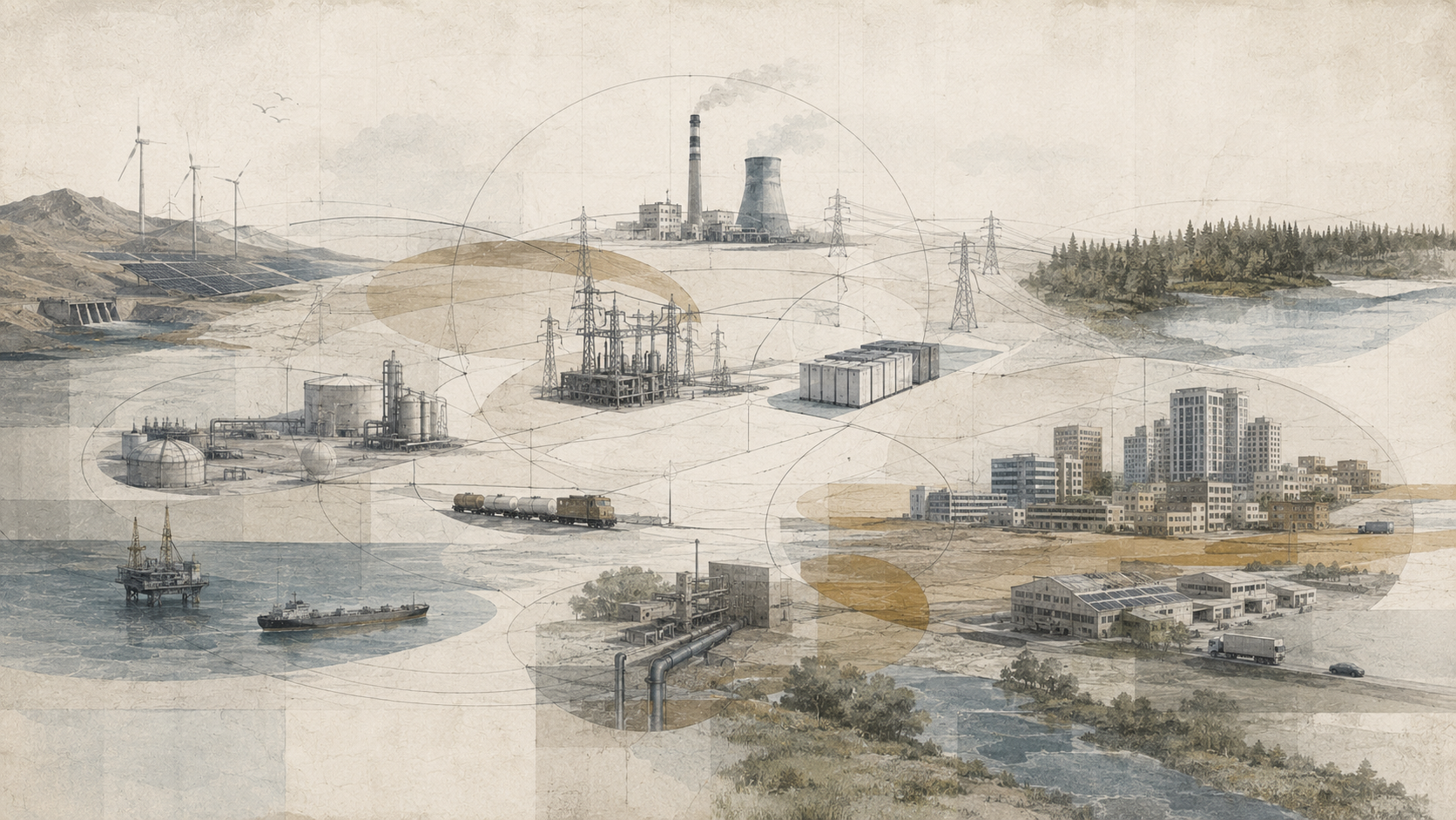
Energy systems are not collections of independent technologies. A power plant depends on fuel, water, finance, regulation, labor, transmission, markets, maintenance, communications, and demand. An electric vehicle depends on electricity generation, charging infrastructure, distribution networks, battery supply chains, roads, consumer behavior, pricing, and public policy. A building’s energy demand depends on climate, architecture, equipment, occupancy, income, codes, utility rates, and cultural expectations. Decisions made in one part of the system can create consequences elsewhere, sometimes years later and far from the original intervention.
Energy systems thinking provides a way to analyze these relationships as interacting structures rather than isolated variables. It asks how components influence one another, how feedback loops reinforce or stabilize change, how delays separate causes from visible effects, how infrastructure and institutions create lock-in, how local optimization can produce system-wide failure, and how interventions can create unintended consequences.
This perspective is especially important during energy transition. Replacing one technology with another is rarely a simple substitution. New generation changes transmission requirements. Electrification changes load shapes. Storage changes dispatch. Efficiency can alter demand through rebound. Climate policy changes investment incentives. New infrastructure creates constituencies and dependencies. Supply-chain constraints can delay deployment. Reliability requirements can change the value of capacity. Public acceptance can determine whether projects are built at all.
Systems thinking does not replace engineering, economics, physics, or policy analysis. It connects them.
The goal is not to make every energy problem more complicated. It is to identify the complexity that materially changes decisions.
Why Energy Needs Systems Thinking
Energy decisions often fail when they optimize a component while ignoring the structure around it.
A utility may add low-cost generation but encounter transmission congestion. A city may subsidize electric vehicles without coordinating distribution upgrades or curbside charging. An efficiency program may reduce the energy required per service while lower operating costs encourage greater use. A region may close dispatchable generation faster than replacement capacity, transmission, storage, or demand flexibility can be built. A fuel policy may shift emissions from one jurisdiction to another without changing global production.
These outcomes are not necessarily caused by bad technology. They arise because the technology is embedded in a larger system.
Systems thinking begins with several questions:
- What are the important components?
- How are they connected?
- What accumulates over time?
- Which feedback loops shape behavior?
- Where are the delays?
- What rules and incentives govern decisions?
- Which actors have power?
- What lies outside the chosen boundary?
- How might the system adapt to intervention?
The purpose is not to map everything. It is to identify enough structure to explain behavior and improve decisions.
Elements, Relationships, and Purpose
A useful systems framework distinguishes among elements, relationships, and system purpose.
Elements are the visible pieces:
- generators;
- transmission lines;
- fuel infrastructure;
- buildings;
- vehicles;
- storage;
- markets;
- regulators;
- consumers;
- ecosystems.
Relationships connect those elements. They include physical flows, prices, information, contracts, legal authority, ownership, technical standards, cultural expectations, and political influence.
Purpose is the function the system actually performs. An electricity system may formally aim to provide reliable power, but its operating rules may also reward particular investments, preserve incumbent assets, recover utility revenue, or prioritize short-run cost minimization. Observed behavior often reveals purposes not stated in mission documents.
Changing elements can matter. Changing relationships or rules can matter more.
Boundaries, Scale, and Perspective
Every system model has a boundary.
An analyst studying a battery may define the system as the cell. A grid planner may include the battery, inverter, feeder, substation, transmission network, generators, and loads. A lifecycle researcher may expand further to mining, manufacturing, transport, recycling, and disposal. A policy analyst may include markets, regulation, communities, and land-use institutions.
The correct boundary depends on the question.
Scale also changes what is visible. An intervention can look beneficial at one level and problematic at another.
| Scale | Typical question | Potentially hidden effects |
|---|---|---|
| Device | How efficient is the technology? | Upstream generation, networks, behavior |
| Building | How does annual energy use change? | Grid peaks, neighborhood constraints |
| Utility | How does load affect system operations? | Regional power transfers, fuel supply |
| Region | How does the portfolio meet demand? | Imported emissions, supply chains |
| Economy | How does energy use affect output and welfare? | Distribution, local ecological impacts |
| Global | How do transitions affect climate and resources? | Local governance, affordability, reliability |
Systems thinking encourages analysts to test whether conclusions survive a change in scale or boundary.
Stocks and Flows
Many energy-system behaviors arise because some quantities accumulate.
A stock is a quantity that exists at a point in time. A flow changes that stock.
Examples of stocks include:
- installed generation capacity;
- battery state of charge;
- fuel inventories;
- building stock;
- vehicle fleet;
- transmission capacity;
- trained workforce;
- atmospheric greenhouse-gas concentration;
- public debt associated with infrastructure.
A generic stock equation is:
S(t+\Delta t)=S(t)+\left(F_{\mathrm{in}}-F_{\mathrm{out}}\right)\Delta t
\]
Stocks change through accumulated inflows and outflows. This simple relationship is foundational to dynamic energy models.
Installed renewable capacity, for example, grows through new construction and falls through retirement:
C_{t+1}=C_t+A_t-R_t
\]
where \(A_t\) is capacity added and \(R_t\) is capacity retired.
This framing prevents a common mistake: treating annual additions as if they were the installed stock. If 10 GW is built in one year, the system does not necessarily gain 10 GW net if 4 GW retires at the same time.
Feedback Loops
A feedback loop occurs when a change in one variable eventually influences itself through a chain of relationships.
Feedback can be reinforcing or balancing.
Reinforcing feedback amplifies change. Balancing feedback counteracts change.
Energy transitions contain both.
For example, larger deployment of a technology can increase manufacturing scale, reduce cost, increase adoption, and create still more deployment. That is a reinforcing loop.
But rapid adoption can also increase demand for scarce materials, raise prices, slow deployment, and reduce the rate of adoption. That is a balancing loop.
The observed trajectory depends on which loops dominate at a particular time.
Reinforcing Feedback
A classic reinforcing loop in energy technology is learning-by-doing:
\text{Deployment}
\rightarrow
\text{Experience}
\rightarrow
\text{Lower Cost}
\rightarrow
\text{Higher Adoption}
\rightarrow
\text{Deployment}
\]
Other reinforcing loops include:
- charging infrastructure increasing electric-vehicle attractiveness, which increases vehicle adoption and encourages more charging investment;
- larger markets encouraging supplier entry, which expands product availability and further increases demand;
- policy support accelerating deployment, which builds political constituencies for continued support;
- network effects that make a technology more useful as adoption grows;
- resource development encouraging infrastructure that lowers the marginal cost of further development.
Reinforcing loops can accelerate beneficial transition, but they can also reinforce harmful systems. Fossil infrastructure, automobile dependence, inefficient building patterns, and institutional practices can become self-reinforcing through the same logic.
Balancing Feedback
Balancing loops resist change.
Consider electricity demand and price:
\text{Demand}
\uparrow
\rightarrow
\text{Price}
\uparrow
\rightarrow
\text{Consumption Response}
\downarrow
\rightarrow
\text{Demand Pressure}
\downarrow
\]
Other balancing mechanisms include:
- resource scarcity increasing costs;
- transmission congestion limiting new generation;
- permitting bottlenecks slowing infrastructure expansion;
- labor shortages constraining construction;
- high adoption reducing remaining market potential;
- grid reliability rules limiting retirement rates;
- public opposition constraining siting;
- higher peak demand triggering efficiency or demand-response investment.
A transition that appears exponential in its early phase may slow when balancing feedback strengthens.
Systems analysis therefore asks not only “What is growing?” but “What will eventually constrain that growth?”
Delays and Dynamic Response
Delays separate action from consequence.
Energy systems contain long delays because infrastructure takes time to permit, finance, manufacture, build, connect, operate, retire, and replace.
Examples include:
- years between transmission planning and energization;
- delays between price signals and new generation investment;
- decades between building-code changes and full turnover of the building stock;
- vehicle-fleet replacement over many years;
- time between workforce investment and available skilled labor;
- long atmospheric residence and climate-system response to greenhouse gases.
Delays can produce overshoot. If investment continues while new capacity remains under construction, the system may eventually receive more capacity than expected. Conversely, if decision makers wait for visible scarcity before acting, projects may arrive too late.
A system can therefore oscillate even when individual actors behave rationally.
The general lesson is that policy should distinguish between the time an intervention is initiated and the time its effects become visible.
Path Dependence and Lock-In
Energy systems are path dependent because previous decisions shape present options.
Once a city is built around highways and dispersed land use, transportation demand reflects that infrastructure. Once buildings use a particular heating fuel, appliances, pipes, codes, contractors, and consumer expectations reinforce the choice. Once a transmission corridor exists, future generation may cluster around it. Once supply chains specialize around a technology, replacement and maintenance become easier than switching systems.
Lock-in can arise through:
- long-lived capital assets;
- sunk cost;
- technical standards;
- network effects;
- professional expertise;
- regulatory structures;
- consumer familiarity;
- political constituencies;
- financing practices;
- land-use patterns.
Lock-in does not mean change is impossible. It means switching costs increase because the system around the technology must change as well.
This is why transition policy often requires coordinated change across infrastructure, standards, finance, workforce, and institutions.
Efficiency and Rebound Effects
Efficiency reduces the energy required to provide a given service. But lower operating cost can change behavior.
Suppose a heating retrofit cuts the energy required per hour of comfortable indoor temperature. If occupants respond by heating more rooms, maintaining higher temperatures, or extending heating hours, some expected savings are offset.
This is a rebound effect.
A simple representation is:
\text{Realized Savings}
=
\text{Engineering Savings}
–
\text{Rebound}
\]
Rebound can occur at several levels:
- Direct rebound: the same service is used more because it becomes cheaper.
- Indirect rebound: money saved is spent on other energy-using goods or services.
- Economy-wide rebound: efficiency changes prices, production, income, investment, and economic structure.
Rebound does not make efficiency useless. It means efficiency outcomes depend on behavioral and economic feedback.
Systems thinking therefore treats demand as endogenous rather than fixed.
Nonlinearity and Thresholds
Many energy relationships are nonlinear.
A transmission line can carry additional flow with little consequence until a limit is reached. Battery degradation can accelerate outside preferred operating ranges. Electricity prices can remain moderate until scarcity causes sharp increases. Reliability can deteriorate rapidly after reserve margins fall below a critical range. Heat-pump performance changes with temperature. Fuel networks may operate smoothly until a compressor, pipeline, or terminal becomes constrained.
In nonlinear systems, doubling an input does not necessarily double the output.
This matters because averages can hide thresholds. A grid that is adequate on average can still fail during a few critical hours. A reservoir that appears secure annually can face seasonal scarcity. A community that tolerates incremental development may oppose a project once cumulative impacts cross a social threshold.
Systems analysis therefore asks where response curves change shape.
Tipping Points and Self-Reinforcing Change
A tipping point occurs when a system crosses a threshold after which feedback drives it toward a different state.
In energy transition, possible tipping dynamics include:
- a technology reaching cost parity and accelerating adoption;
- charging infrastructure becoming dense enough to reduce consumer range concerns;
- a declining incumbent market raising unit costs for remaining customers, accelerating further departures;
- supplier ecosystems reaching enough scale to support rapid diffusion;
- political coalitions shifting as employment and investment move between industries.
Not every rapid change is a tipping point, and not every threshold is irreversible. The concept should be used carefully.
A useful analytical test is to ask whether crossing the threshold changes the dominant feedback structure. If the system begins reinforcing the new state without continuing external intervention, tipping language may be appropriate.
Interdependence Across Energy Sectors
Energy sectors increasingly interact.
Electricity can power vehicles, heat buildings, produce hydrogen, operate industrial processes, run data centers, and support water systems. Natural gas can supply power generation and buildings while also serving as industrial feedstock. Hydrogen can link electricity, fuels, refining, fertilizer, steel, storage, and transport.
Electrification therefore creates cross-sector coupling.
A heat wave may simultaneously:
- increase air-conditioning demand;
- reduce thermal-plant efficiency;
- constrain hydropower or cooling water;
- stress distribution transformers;
- increase wildfire risk near transmission;
- raise public-health consequences of outages.
Analyzing only one sector can miss these compound effects.
Coupled Infrastructure Systems
Energy depends on other infrastructures, and those infrastructures depend on energy.
Electricity powers:
- water pumping and treatment;
- communications;
- health care;
- transportation control;
- fuel terminals;
- data centers;
- financial systems;
- emergency services.
At the same time, electricity systems depend on communications, transportation, water, fuel delivery, and digital control.
These dependencies create the possibility of cascading failure.
A power outage can disable communications. Communications loss can impede grid restoration. Fuel stations may be unable to pump fuel. Transportation disruptions can delay repair crews. Water systems may lose pressure. Hospitals may depend on backup generators whose fuel supply is constrained.
Resilience planning should therefore map interdependencies rather than treat critical infrastructures separately.
Institutions, Markets, and Rules
Energy systems are governed systems.
Markets determine dispatch, investment, and revenue. Regulators determine allowable rates and cost recovery. Building codes influence demand. Interconnection rules influence distributed generation. Permitting affects transmission and generation. Tax policy changes investment incentives. Reliability standards shape reserve requirements. Public utility structures determine ownership and accountability.
Rules create feedback.
For example, a utility revenue model based primarily on volumetric sales may discourage aggressive efficiency because lower consumption reduces revenue. A performance-based model can change that incentive. A capacity market can reward availability that an energy-only market may undervalue. Interconnection queues can slow projects even when technology costs are low.
Systems thinking therefore treats policy as part of system structure rather than as an external correction applied afterward.
Behavior, Demand, and Social Practice
Energy demand is not produced only by devices. It emerges from social practices.
Mobility demand depends on land use, work patterns, transit availability, household structure, and expectations about distance. Heating demand depends on building quality, climate, occupancy, clothing, comfort expectations, and affordability. Data-center demand depends on computing architecture, service growth, hardware efficiency, and business models.
This matters because technology alone may not determine consumption.
A more efficient vehicle can reduce energy per kilometer while longer travel distances offset the gain. Better insulation can reduce heating demand, but larger floor area can offset part of the saving. Efficient servers can reduce energy per computation while computational demand grows much faster.
Systems thinking asks how technology changes the service itself.
Resilience and Adaptation
A resilient energy system can absorb disruption, adapt, and recover while maintaining essential functions.
Resilience arises from multiple forms of capacity:
- redundancy;
- diverse resources;
- spare capacity;
- storage;
- islanding;
- mutual assistance;
- repair capability;
- distributed control;
- fuel diversity;
- adaptive operating procedures.
Some of these features appear inefficient under narrow utilization metrics. Redundant infrastructure may sit idle. Reserve capacity may rarely run. Spare transformers occupy inventory. But these resources create value under disturbance.
Systems thinking distinguishes efficiency from resilience. A system optimized to eliminate all slack may become fragile.
The design question is not whether redundancy is wasteful, but how much redundancy is justified by the consequences and probability of failure.
Unintended Consequences
Interventions often create second-order effects.
Examples include:
- efficiency lowering operating cost and increasing use;
- distributed generation reducing utility sales and shifting fixed network costs;
- rapid electrification increasing local distribution constraints;
- cheap electricity stimulating new energy-intensive demand;
- subsidies accelerating adoption but creating boom-and-bust installation cycles when withdrawn;
- strict local environmental rules shifting production elsewhere;
- biofuel demand affecting land, food markets, and ecosystems;
- hydrogen policy increasing electricity demand and transmission requirements.
The existence of unintended consequences does not imply that intervention should be avoided. It means policy should anticipate system response.
A useful question is:
What will actors do differently after the intervention changes prices, constraints, information, or incentives?
Leverage Points
A leverage point is a place where a relatively small intervention can produce a large system effect.
Not all leverage points are equally powerful.
Changing a parameter such as a subsidy rate can matter, but changing information flows, institutional rules, incentives, or system goals may have deeper effects.
In energy systems, leverage points can include:
- interconnection rules;
- transmission planning authority;
- building standards;
- rate design;
- market settlement rules;
- procurement standards;
- public access to operational data;
- ownership structures;
- permitting coordination;
- planning assumptions about demand and reliability.
A powerful leverage point can also generate resistance. Changing rules redistributes costs, benefits, authority, and risk.
Systems analysis should therefore pair technical leverage with institutional feasibility.
Causal-Loop Diagrams
A causal-loop diagram maps hypothesized relationships among variables.
A positive link means that, all else equal, an increase in one variable tends to increase the next relative to what it otherwise would have been. A negative link means an increase tends to reduce the next variable.
Consider renewable deployment:
\text{Deployment}
\xrightarrow{+}
\text{Experience}
\xrightarrow{+}
\text{Productivity}
\xrightarrow{-}
\text{Cost}
\xrightarrow{-}
\text{Adoption Barrier}
\xrightarrow{-}
\text{Deployment}
\]
The overall loop is reinforcing because the sequence of negative and positive relationships ultimately amplifies deployment.
A causal-loop diagram should not be treated as proof. It is a structured hypothesis about causation.
Good practice includes:
- using measurable variables where possible;
- avoiding ambiguous labels such as “better policy”;
- distinguishing correlation from causation;
- showing delays;
- identifying evidence for important links;
- testing whether omitted variables change conclusions.
Stock-and-Flow Models
Causal-loop diagrams describe structure qualitatively. Stock-and-flow models make accumulation explicit and can simulate change through time.
Suppose renewable capacity changes through additions and retirements:
\frac{dC}{dt}=A(t)-R(t)
\]
Additions may depend on profitability, policy, manufacturing capacity, interconnection, and permitting:
A(t)=f\left(P_t,\ K_t,\ Q_t,\ M_t,\ \tau_t\right)
\]
where:
- \(P_t\) = project economics;
- \(K_t\) = manufacturing capacity;
- \(Q_t\) = interconnection availability;
- \(M_t\) = material availability;
- \(\tau_t\) = permitting and construction delay.
Retirements may depend on age, economics, reliability requirements, and policy.
This structure allows a model to reproduce dynamics that static scenario tables cannot.
Scenario Analysis and Deep Uncertainty
Energy systems contain uncertainty that cannot always be represented by one probability distribution.
Future technology costs, political decisions, climate impacts, public acceptance, demand growth, fuel prices, supply-chain conditions, and geopolitical events may be deeply uncertain.
Scenario analysis explores multiple internally coherent futures rather than pretending one forecast is certain.
A systems-oriented scenario framework can vary:
- demand growth;
- electrification rate;
- technology learning;
- fuel prices;
- transmission build rate;
- storage cost;
- permitting duration;
- climate extremes;
- material constraints;
- policy durability;
- consumer adoption;
- retirement schedules.
The purpose is not to identify the “correct” future. It is to identify strategies that remain acceptable across several plausible futures.
This shifts planning from prediction toward robustness.
Worked Examples
Example 1: Capacity Stock with Retirements
A region begins with 40 GW of renewable capacity. During the year, 8 GW is added and 3 GW retires.
C_{t+1}=40+8-3=45\ \mathrm{GW}
\]
Annual additions are 8 GW, but the stock grows by only 5 GW.
Example 2: Learning Feedback
Suppose cumulative deployment doubles and a technology experiences a 20 percent learning rate. Cost falls to:
C_{\mathrm{new}}=C_{\mathrm{old}}(1-0.20)=0.80C_{\mathrm{old}}
\]
If lower cost increases adoption, the next deployment increment may accelerate another cost reduction. The relationship becomes reinforcing.
Example 3: Delay and Overshoot
A region needs 5 GW of additional firm capacity. Projects take four years to build. Decision makers continue ordering 2 GW per year until completed capacity becomes visible.
By the time the first 2 GW arrives, 8 GW may already be in the pipeline. The delay creates the possibility of overbuilding even if each annual decision responded rationally to the visible shortage.
Example 4: Rebound
An efficiency upgrade is expected to reduce household heating demand from 20 MWh to 14 MWh annually: an engineering saving of 6 MWh.
After the retrofit, occupants increase comfort and actual demand is 15.5 MWh.
Realized savings are:
20-15.5=4.5\ \mathrm{MWh}
\]
The rebound is:
6-4.5=1.5\ \mathrm{MWh}
\]
or 25 percent of the expected engineering saving.
Example 5: Coupled Infrastructure Failure
A severe storm disconnects a substation serving a water-treatment facility. The treatment plant switches to backup generation, but road flooding delays fuel delivery. Communications outages reduce coordination, while low water pressure complicates emergency response.
No single infrastructure failure explains the outcome. The disruption emerges from dependencies among power, transport, fuel, communications, water, and emergency services.
That is a systems problem.
Common Misconceptions
Misconception 1: Systems thinking means everything affects everything.
Useful systems analysis identifies important causal structure, not unlimited complexity.
Misconception 2: A system map is automatically a model.
A map can organize thinking, but quantitative models require equations, data, assumptions, and validation.
Misconception 3: Feedback is always positive or desirable.
“Positive” feedback means reinforcing, not beneficial. “Negative” feedback means balancing, not harmful.
Misconception 4: Rebound eliminates efficiency gains.
Rebound can offset part of an efficiency improvement, but its magnitude varies by service, price, income, and context.
Misconception 5: Lock-in means change is impossible.
Lock-in means the existing system creates switching costs and reinforcing structures.
Misconception 6: More detail always improves a model.
Excess detail can obscure causation, increase uncertainty, and make models harder to validate.
Misconception 7: A leverage point guarantees easy change.
High-leverage interventions often challenge incumbent interests and institutional rules.
Python Workflow: Feedback and Capacity Dynamics
A simple dynamic model can represent installed capacity, deployment, learning, and retirement.
from dataclasses import dataclass

@dataclass
class State:
    year: int
    capacity_gw: float
    cumulative_build_gw: float
    unit_cost: float

learning_rate = 0.18
retirement_rate = 0.025
base_build = 5.0

state = State(
    year=2026,
    capacity_gw=40.0,
    cumulative_build_gw=80.0,
    unit_cost=100.0,
)

history = []

for _ in range(20):
    # Lower cost increases annual build.
    build = base_build * (100.0 / state.unit_cost)

    retirements = state.capacity_gw * retirement_rate

    old_cumulative = state.cumulative_build_gw
    new_cumulative = old_cumulative + build

    # Learning curve:
    # cost scales with cumulative deployment.
    exponent = (
        __import__("math").log2(1.0 - learning_rate)
    )
    new_cost = 100.0 * (
        new_cumulative / 80.0
    ) ** exponent

    state = State(
        year=state.year + 1,
        capacity_gw=state.capacity_gw + build - retirements,
        cumulative_build_gw=new_cumulative,
        unit_cost=new_cost,
    )

    history.append(state)

for row in history:
    print(
        row.year,
        round(row.capacity_gw, 2),
        round(row.unit_cost, 2),
    )
This model is deliberately simple. It demonstrates a reinforcing learning loop combined with a balancing retirement flow.
A more realistic model could add:
- manufacturing limits;
- material constraints;
- permitting queues;
- interconnection delays;
- transmission availability;
- financing conditions;
- demand growth;
- policy changes;
- capacity-factor differences;
- regional interactions.
The value of the model lies in making assumptions explicit enough to test.
R Workflow: Scenario Comparison
R can compare how different feedback and constraint assumptions alter system trajectories.
scenarios <- data.frame(
  scenario = c(
    "Coordinated build",
    "Transmission constrained",
    "Slow permitting",
    "Rapid learning"
  ),
  annual_build_gw = c(8, 5, 4, 10),
  retirement_gw = c(3, 3, 3, 3),
  years = c(10, 10, 10, 10)
)

scenarios$net_addition_gw <-
  scenarios$annual_build_gw -
  scenarios$retirement_gw

scenarios$capacity_change_gw <-
  scenarios$net_addition_gw *
  scenarios$years

print(scenarios)
A richer model could make annual build endogenous rather than fixed, with deployment responding to cost, permitting, transmission, manufacturing, and policy.
Scenario comparison is useful when no single forecast deserves complete confidence. The objective is to understand which constraints dominate and which interventions remain useful across alternative futures.
GitHub Repository
Complete Code Repository
The full Energy Systems repository contains reproducible article workflows, stock-and-flow models, feedback-loop examples, scenario analysis, sensitivity methods, energy-accounting tools, datasets, documentation, and multi-language computational assets.
A Practical Systems-Thinking Method
A rigorous energy-systems study can follow a repeatable sequence:
- Define the decision. State what choice, risk, or behavior the analysis should illuminate.
- Set the boundary. Identify geography, sectors, time horizon, infrastructure, actors, and external systems.
- Identify key stocks. Determine what accumulates: capacity, vehicles, buildings, inventories, emissions, workforce, capital, or public support.
- Identify flows. Map additions, retirements, charging, discharge, investment, adoption, extraction, and other rates of change.
- Map causal relationships. Document how variables influence one another.
- Identify reinforcing loops. Look for learning, network effects, scale economies, and self-reinforcing adoption.
- Identify balancing loops. Look for scarcity, congestion, price response, regulation, physical limits, and opposition.
- Mark delays. Separate decision time, construction time, response time, and turnover time.
- Test lock-in. Identify standards, sunk assets, infrastructure, institutions, and behavioral patterns that make switching difficult.
- Look for rebound. Ask how lower cost or higher efficiency changes demand.
- Identify thresholds. Find operating limits, saturation points, capacity constraints, and possible tipping dynamics.
- Map interdependencies. Include water, communications, transport, finance, supply chains, and public institutions where material.
- Quantify what matters. Convert the most important relationships into equations or simulation rules.
- Build scenarios. Test multiple futures rather than one deterministic forecast.
- Validate behavior. Compare model dynamics with historical data, engineering constraints, and expert knowledge.
- Identify leverage points. Focus on interventions capable of changing system structure rather than only symptoms.
A strong systems analysis should be understandable enough that another analyst can challenge the map, modify assumptions, and reproduce the main conclusions.
Policy, Equity, and Public Value
Energy systems distribute benefits, costs, authority, and risk.
A technically efficient intervention can still create inequitable outcomes if costs are shifted to low-income customers, infrastructure is concentrated in overburdened communities, benefits accrue primarily to asset owners, or essential services become less affordable.
Systems thinking helps make distribution visible.
Questions of public value include:
- Who pays for infrastructure?
- Who receives the reliability benefit?
- Who bears environmental and land-use burdens?
- Who controls investment decisions?
- Which customers can respond to dynamic prices?
- Who can afford new technologies?
- Which communities are vulnerable to outages?
- Which workers and regions depend on incumbent industries?
- How are transition risks shared?
These are not external social questions added after technical optimization. They can alter adoption, siting, political durability, financing, and system performance.
Legitimacy is part of system capacity.
Limits, Uncertainty, and Responsible Interpretation
Systems thinking can become vague if every relationship is described qualitatively without evidence.
Common risks include:
- drawing causal arrows that are only correlations;
- expanding the boundary until the model becomes unusable;
- using feedback language without specifying measurable variables;
- assuming all relationships are stable over time;
- ignoring actor strategy and institutional power;
- treating simulation output as prediction;
- hiding uncertainty behind model complexity;
- failing to test model behavior against real observations.
Responsible practice should distinguish among:
Observed relationships, supported by data.
Mechanistic relationships, supported by physics or engineering.
Behavioral relationships, supported by empirical evidence but subject to context.
Hypothesized relationships, included for scenario testing.
Models should also separate uncertainty in parameters from uncertainty in structure. A precise estimate of a parameter does not solve uncertainty about whether the model includes the right causal relationships.
The objective is disciplined simplification.
From Components to Systems
Energy systems thinking changes the unit of analysis.
Instead of asking only whether a technology works, it asks what happens when the technology interacts with infrastructure, markets, institutions, behavior, ecology, and other technologies. Instead of asking only how much capacity is built, it asks how stocks change after retirements and delays. Instead of assuming efficiency automatically reduces demand, it examines rebound. Instead of assuming cost declines guarantee deployment, it examines transmission, permitting, supply chains, and public acceptance.
The central insight is that system behavior emerges from structure.
Feedback loops can accelerate or constrain transition. Delays can create overshoot and shortage. Long-lived assets and standards create path dependence. Coupled infrastructures create cascading risk. Market rules and institutions shape investment. Behavior changes in response to technology and prices. Thresholds can turn gradual pressure into rapid change.
Systems thinking does not eliminate uncertainty, and it does not produce a single master model of the energy system. Its value is practical: it helps analysts identify which relationships materially change decisions, where interventions may create second-order effects, and where leverage lies.
This article completes the foundational opening sequence of the Energy Systems series. The next section moves into electricity and grid systems, beginning with Electricity Grids: generation, transmission, distribution, balancing, frequency, voltage, reliability, and system operation.
Related Articles
- What Are Energy Systems?
- Energy, Power, and Work
- Energy and Thermodynamics
- Primary, Secondary, and Final Energy
- Energy Flows and Sankey Diagrams
- Energy Return on Investment
- Electricity Grids
- Grid Reliability and Resilience
Further Reading
- Meadows, Donella H. Thinking in Systems: A Primer.
- Forrester, Jay W. Foundational work in system dynamics.
- Sterman, John D. Business Dynamics: Systems Thinking and Modeling for a Complex World.
- Meadows, Donella H. “Leverage Points: Places to Intervene in a System.”
- International Energy Agency. Energy-system transition and infrastructure analysis.
- Intergovernmental Panel on Climate Change. Energy-system transformation, mitigation pathways, and institutional context.
- National laboratories and system operators. Grid planning, reliability, resilience, and transition studies.
References
- Meadows, Donella H. Thinking in Systems: A Primer. Chelsea Green Publishing.
- Meadows, Donella H. “Leverage Points: Places to Intervene in a System.” Sustainability Institute.
- Forrester, Jay W. Industrial Dynamics. MIT Press.
- Sterman, John D. Business Dynamics: Systems Thinking and Modeling for a Complex World. McGraw-Hill.
- International Energy Agency. Energy system analysis and transition resources. Available at: IEA.
- Intergovernmental Panel on Climate Change. Climate Change 2022: Mitigation of Climate Change. Available at: IPCC.
- U.S. Department of Energy. Grid modernization, resilience, and systems research. Available at: DOE.
- National Renewable Energy Laboratory. Energy systems integration and power-system research. Available at: NREL.