Genomics, Sequence Analysis, and Biological Data

Last Updated May 28, 2026

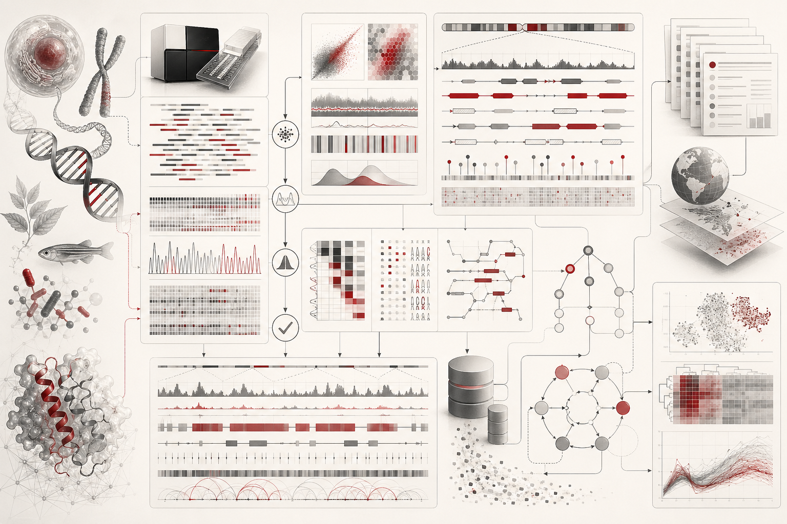
Genomics, sequence analysis, and biological data define one of the central knowledge infrastructures of modern life science: the ability to read, compare, annotate, store, validate, interpret, and responsibly reuse the molecular information encoded in DNA, RNA, proteins, genomes, transcriptomes, metagenomes, and biological variation. Genomics is not only the study of genes or genome sequences. It is a computational, statistical, molecular, evolutionary, and infrastructural field that connects biological material to digital records, digital records to analysis, and analysis to scientific claims.

This article introduces genomics and sequence analysis as foundations of contemporary biology. It explains how sequence data move from biological samples to sequencing instruments, from instruments to reads, from reads to files, from files to alignments and assemblies, from assemblies to annotation, from annotation to biological interpretation, and from interpretation to reusable scientific knowledge. Genomic data are never merely strings of letters. They are measured, processed, filtered, annotated, versioned, stored, compared, and interpreted through scientific workflows.

The article is written for biologists, ecologists, marine biologists, biomedical researchers, genomics scientists, laboratory scientists, computational biologists, bioinformaticians, systems biologists, biotechnology teams, data engineers, environmental scientists, and engineers who need to understand how sequence data become biological evidence. It connects molecular biology, sequencing technologies, FASTA and FASTQ logic, reference genomes, alignment, assembly, annotation, variant representation, metadata, quality control, data repositories, reproducibility, and responsible interpretation.

The article also extends the discussion into reproducible computational practice through sequence parsing, GC-content analysis, k-mer counting, open reading frame detection, simple translation scaffolds, FASTQ-style quality summaries, metadata validation, variant-table checks, SQL-backed provenance, Python and R examples, and a linked full-stack GitHub repository containing Python, R, Julia, Fortran, Rust, Go, C, C++, SQL, notebooks, data files, validation notes, and reproducibility documentation.

Why genomics matters

Genomics matters because it allows biology to be studied through the molecular information systems that organisms inherit, regulate, modify, express, and evolve. DNA sequence, RNA sequence, protein sequence, genome structure, gene regulation, mutation, recombination, horizontal gene transfer, mobile elements, chromatin organization, and genomic variation all provide evidence about how living systems function and change.

A genome is not merely a catalog of genes. It is a structured biological archive shaped by evolutionary history, molecular constraint, regulatory architecture, environmental pressure, population dynamics, and cellular machinery. A genome contains coding sequences, regulatory regions, repeats, structural variants, noncoding RNAs, transposable elements, conserved regions, lineage-specific changes, and many regions whose functions remain uncertain.

Genomics therefore changes the scale of biological inquiry. It allows researchers to compare organisms, identify genes, infer evolutionary relationships, detect variation, study disease mechanisms, track pathogens, monitor biodiversity, analyze microbial communities, reconstruct phylogenies, examine adaptation, and connect molecular systems to ecological and biomedical questions.

But genomics also changes the responsibilities of biology. Sequence data require computational literacy, metadata discipline, file-format awareness, quality control, repository practice, privacy safeguards, and reproducible workflows. Genomics expands biological knowledge only when data remain interpretable.

Back to top ↑

Sequence data as biological evidence

Sequence data may look simple because they are often represented as strings of letters: A, C, G, T for DNA; A, C, G, U for RNA; and amino-acid symbols for proteins. But sequence data are not simple. They are produced by instruments, protocols, library preparations, base-calling algorithms, filtering rules, reference choices, annotation pipelines, and statistical assumptions.

A sequence read is not the same as a genome. A read is an observed fragment, with uncertainty. A genome assembly is a computational reconstruction. A gene annotation is an interpretation layered onto a sequence. A variant call is an inference based on evidence, thresholds, reference coordinates, read depth, mapping quality, and model assumptions.

This matters because sequence data can mislead if treated as self-explanatory. Contamination, low-quality reads, adapter sequences, poor assembly, reference bias, sample swaps, batch effects, incomplete metadata, repetitive regions, paralogs, sequencing errors, and algorithmic artifacts can all distort inference.

Good sequence analysis therefore treats genomic data as evidence with provenance. It asks: What biological material was sequenced? Which technology was used? What quality scores were observed? Which reference was used? Which version? Which parameters? Which filters? Which annotations? Which database? Which assumptions?

Back to top ↑

From sample to sequence

A genomics workflow begins before sequencing. It begins with biological sampling. Tissue, blood, saliva, soil, seawater, microbial culture, tumor material, plant leaf, environmental DNA, single cells, or ancient material each carries different constraints. Sampling affects representation, contamination risk, degradation, yield, and interpretation.

After sampling, nucleic acids are extracted, prepared, and sequenced. Library preparation may involve fragmentation, amplification, barcoding, adapter ligation, enrichment, size selection, or capture. Sequencing technologies then generate reads, which are transformed through base calling into digital sequence files.

Each step shapes the data. Low-quality extraction can fragment DNA. PCR can introduce bias. Barcoding errors can misassign reads. Short-read sequencing may struggle with repetitive regions. Long-read sequencing may improve structural resolution but require different error handling. Single-cell sequencing may introduce dropout and amplification bias. Metagenomic sequencing may contain mixed organisms and uneven abundance.

A responsible genomics workflow records these details. Sequence data are meaningful only when connected to sample identity, protocol, instrument, date, batch, quality metrics, and biological context.

Back to top ↑

FASTA, FASTQ, and the logic of sequence files

FASTA and FASTQ are foundational sequence-file formats. FASTA represents sequence records with identifiers and sequence strings. It is commonly used for reference sequences, assembled contigs, transcripts, proteins, primers, and teaching examples. FASTQ extends sequence representation by including per-base quality scores, making it central to raw sequencing-read workflows.

The key distinction is uncertainty. FASTA often represents a sequence as accepted or assembled. FASTQ represents reads with quality information. A nucleotide in a FASTQ file is not simply a letter; it is a base call associated with a quality score. That score reflects confidence in the call.

File formats also carry identifiers. A sequence identifier can connect reads to samples, contigs to assemblies, genes to annotations, variants to references, and records to repositories. If identifiers are inconsistent, downstream analysis becomes fragile.

Sequence analysis therefore begins with file discipline: valid format, unique identifiers, clear naming conventions, controlled metadata, versioned references, and reproducible parsing.

Back to top ↑

Quality control and sequencing error

Sequencing data require quality control because sequencing is measurement, not transcription from nature. Reads may contain base-call errors, adapter contamination, low-quality tails, short fragments, duplicates, overrepresented sequences, biased GC content, index hopping, contamination, and platform-specific artifacts.

Quality control asks whether the data are fit for the intended analysis. For read data, this may include read length distribution, per-base quality, GC-content distribution, duplication rate, adapter content, ambiguous bases, mapping rate, coverage, and contamination screening. For assemblies, this may include contiguity, completeness, misassembly detection, contamination, and annotation consistency. For variant calls, this may include read depth, mapping quality, allele balance, genotype quality, and filtering thresholds.

Quality control is not a cosmetic step. It shapes inference. Removing low-quality reads may improve reliability but can also alter representation. Filtering variants may reduce false positives but remove true signals. Trimming reads may improve alignment but shorten useful sequence. Every quality decision should be documented.

Back to top ↑

Alignment, assembly, and reference genomes

Alignment places sequences in relation to other sequences. Reads may be aligned to a reference genome. Proteins may be aligned to infer conserved domains. Gene sequences may be aligned to compare species. Alignment helps identify similarity, difference, structure, and evolutionary relationship.

Reference-based analysis depends heavily on the reference genome. The reference provides coordinates, gene models, annotation context, and a framework for variant calling. But references can introduce bias, especially when samples differ substantially from the reference lineage, when structural variation is present, or when populations are underrepresented in reference construction.

Assembly reconstructs longer sequences from reads. De novo assembly attempts to build sequences without relying entirely on a reference. Assembly is essential for novel organisms, metagenomics, structural variation, microbial genomics, and many ecological or evolutionary contexts. But assembly is difficult because repeats, heterozygosity, contamination, uneven coverage, and sequencing error can create ambiguity.

A genomic coordinate is therefore not just a location. It is a location relative to a specific reference assembly and annotation version. Responsible sequence analysis always records reference identity and version.

Back to top ↑

Annotation and biological meaning

Annotation connects sequence to biological meaning. It identifies genes, transcripts, exons, introns, regulatory regions, protein-coding regions, noncoding RNAs, repeats, domains, motifs, variants, pathways, and functional predictions. Annotation transforms a sequence from a string into a biological map.

But annotation is not the same as fact. Some annotations are experimentally supported. Others are computational predictions. Some are curated manually. Others are transferred from homologous sequences. Some gene models are stable. Others change as assemblies improve, transcript evidence expands, or functional knowledge advances.

This is why annotation versioning matters. A gene name, transcript ID, or genomic coordinate may change between releases. A variant can appear different if mapped to another reference. A transcript can be reclassified. A predicted function can be revised.

Sequence analysis should therefore distinguish sequence, coordinate, annotation, evidence, and interpretation. Genomic data become scientifically useful when these layers remain traceable.

Back to top ↑

Variation and genomic difference

Genomic variation includes single-nucleotide variants, insertions, deletions, copy-number variants, inversions, translocations, repeat expansions, mobile-element insertions, structural variants, and differences in gene content. Variation is central to evolution, disease, adaptation, population structure, inheritance, biodiversity, and biotechnology.

Variant analysis depends on reference context. A variant is usually described relative to a reference sequence and coordinate system. This means that reference version, genome build, transcript model, and normalization rules matter. Ambiguous representation can make variants difficult to compare across datasets.

Variation also requires biological interpretation. A variant may be synonymous, missense, nonsense, regulatory, structural, pathogenic, benign, adaptive, neutral, population-specific, somatic, germline, inherited, de novo, or uncertain. Evidence matters. Context matters. Frequency matters. Functional validation matters.

Genomic difference is therefore not just a computational output. It is a biological claim requiring evidence, representation, metadata, and careful interpretation.

Back to top ↑

Metadata, provenance, and repositories

Sequence data gain scientific value when they are connected to metadata and deposited in reliable repositories. Metadata may include organism, sample source, tissue, location, collection date, project, library strategy, sequencing platform, instrument, reference genome, assembly version, study design, phenotype, environment, and consent or access restrictions where relevant.

Provenance records how data were produced and transformed. It connects raw reads to quality-control steps, trimmed reads, alignments, assemblies, annotations, variant calls, summary tables, figures, and reports. Without provenance, genomic results can be difficult to reproduce or audit.

Repositories such as GenBank, SRA, ENA, and related systems form the public infrastructure of sequence biology. They allow sequence data to be preserved, searched, cited, compared, and reused. They also require standards, identifiers, validation, and submission discipline.

The future value of sequence data depends on this infrastructure. A genome sequence without metadata may become nearly unusable. A well-documented sequence dataset can support new science long after its original publication.

Back to top ↑

Comparative genomics and evolutionary inference

Comparative genomics uses sequence similarity and difference to infer biological relationships. It can identify conserved genes, lineage-specific expansions, gene loss, horizontal gene transfer, adaptive evolution, synteny, regulatory conservation, structural rearrangements, and evolutionary novelty.

Sequence similarity tools such as BLAST help identify local similarity between biological sequences and support functional and evolutionary inference, but similarity is not identical to function. Homology, orthology, paralogy, convergence, domain architecture, and gene duplication complicate interpretation.

Comparative genomics is powerful because evolution leaves molecular traces. But inference requires caution. A gene may be similar because of shared ancestry. A domain may be conserved while function diverges. A sequence may match a contaminant. A database hit may be biased by overrepresented organisms. Absence from a database does not prove absence from life.

The strongest comparative genomics combines sequence analysis with phylogeny, annotation, expression, structure, ecology, and experimental evidence.

Back to top ↑

Genomics in ecology, medicine, and biotechnology

Genomics now reaches across biology. In ecology, environmental DNA, metagenomics, population genomics, and conservation genomics help monitor biodiversity, detect invasive species, study microbial communities, and infer adaptation. In medicine, genomics supports rare disease diagnosis, cancer profiling, pathogen surveillance, pharmacogenomics, and inherited-risk analysis. In biotechnology, genomics supports strain engineering, synthetic biology, enzyme discovery, genome editing, agricultural improvement, and biomarker development.

Each domain has different data responsibilities. Ecological genomics must attend to sampling context, contamination, environmental metadata, and taxonomic uncertainty. Medical genomics must attend to privacy, consent, clinical validity, variant interpretation, and governance. Biotechnology must attend to reproducibility, biosafety, design traceability, and functional validation.

The common requirement is disciplined data practice. Genomic data are powerful because they can travel across contexts, but that same portability creates risk when metadata, consent, provenance, reference context, or uncertainty are lost.

Back to top ↑

Mathematical lens: sequence analysis

Several mathematical ideas are central to genomics and sequence analysis. These expressions do not replace molecular biology, laboratory evidence, evolutionary interpretation, or clinical judgment. They help clarify how sequence length, base composition, k-mer patterns, distance, quality, coverage, and variant support can be represented formally.

Sequence length

GC content

K-mer count

Hamming distance

Edit distance

Phred quality score

Coverage

Variant allele frequency

Back to top ↑

Python and R workflows

The following examples are compact article-level workflows. The full GitHub repository expands them into richer full-stack implementations with SQL provenance, cross-language validation, sequence summaries, quality-control checks, variant-table validation, and reproducible project documentation.

Python example: FASTA parsing and sequence summary

from collections import Counter
import pandas as pd

VALID_DNA = {"A", "C", "G", "T"}

def parse_fasta_text(fasta_text: str) -> dict[str, str]:
    """Parse a small FASTA string into sequence records."""
    records = {}
    current_id = None
    current_sequence = []

    for line in fasta_text.strip().splitlines():
        line = line.strip()

        if line.startswith(">"):
            if current_id is not None:
                records[current_id] = "".join(current_sequence).upper()
            current_id = line[1:].split()[0]
            current_sequence = []
        else:
            current_sequence.append(line)

    if current_id is not None:
        records[current_id] = "".join(current_sequence).upper()

    return records

def gc_content(sequence: str) -> float:
    valid_bases = [base for base in sequence.upper() if base in VALID_DNA]
    counts = Counter(valid_bases)

    if len(valid_bases) == 0:
        return float("nan")

    return (counts["G"] + counts["C"]) / len(valid_bases)

fasta_text = """
>sample_01
ATGCGCGTAATTAACCGGTTACCGTAGCTA
>sample_02
ATATATGGCCNNATGCGTAACCGGTTAACTA
"""

records = parse_fasta_text(fasta_text)

summary = pd.DataFrame(
    {
        "sequence_id": sequence_id,
        "length": len(sequence),
        "gc_content": gc_content(sequence),
        "ambiguous_bases": sum(base not in VALID_DNA for base in sequence.upper()),
    }
    for sequence_id, sequence in records.items()
)

print(summary.round(4).to_string(index=False))

Python example: k-mer counting

from collections import Counter

def count_kmers(sequence: str, k: int) -> Counter:
    """Count valid DNA k-mers in a sequence."""
    sequence = sequence.upper()
    valid = {"A", "C", "G", "T"}
    counts = Counter()

    for start in range(len(sequence) - k + 1):
        kmer = sequence[start:start + k]
        if set(kmer).issubset(valid):
            counts[kmer] += 1

    return counts

sequence = "ATGCGCGTAATTAACCGGTTACCGTAGCTA"
counts = count_kmers(sequence, k=3)

for kmer, count in counts.most_common(10):
    print(kmer, count)

Python example: open reading frame scaffold

STOP_CODONS = {"TAA", "TAG", "TGA"}

def find_simple_orfs(sequence: str, minimum_codons: int = 3) -> list[dict]:
    """Find simple ATG-to-stop open reading frames on the forward strand."""
    sequence = sequence.upper()
    orfs = []

    for frame in range(3):
        start = None

        for position in range(frame, len(sequence) - 2, 3):
            codon = sequence[position:position + 3]

            if codon == "ATG" and start is None:
                start = position

            if codon in STOP_CODONS and start is not None:
                codon_length = (position + 3 - start) // 3

                if codon_length >= minimum_codons:
                    orfs.append(
                        {
                            "frame": frame,
                            "start": start,
                            "end": position + 3,
                            "codons": codon_length,
                            "stop_codon": codon,
                        }
                    )

                start = None

    return orfs

sequence = "CCCATGAAACCCGGGTAGCCCATGTTTTAA"
print(find_simple_orfs(sequence, minimum_codons=3))

Python example: variant table validation

import pandas as pd

variants = pd.DataFrame(
    {
        "chromosome": ["chr1", "chr1", "chr2"],
        "position": [1050, 1088, 2201],
        "reference": ["A", "G", "T"],
        "alternate": ["G", "A", "C"],
        "read_depth": [42, 31, 8],
        "alternate_depth": [18, 3, 4],
    }
)

valid_bases = {"A", "C", "G", "T"}

variants["valid_ref_alt"] = variants.apply(
    lambda row: row["reference"] in valid_bases and row["alternate"] in valid_bases,
    axis=1,
)

variants["variant_allele_frequency"] = (
    variants["alternate_depth"] / variants["read_depth"]
)

variants["passes_depth_threshold"] = variants["read_depth"] >= 10

print(variants.round(4).to_string(index=False))

R example: sequence summary cross-check

# Compact R sequence summary cross-check.

sequence_table <- data.frame(
  sequence_id = c("sample_01", "sample_02"),
  sequence = c(
    "ATGCGCGTAATTAACCGGTTACCGTAGCTA",
    "ATATATGGCCNNATGCGTAACCGGTTAACTA"
  )
)

gc_content <- function(sequence) {
  bases <- strsplit(toupper(sequence), "")[[1]]
  valid <- bases[bases %in% c("A", "C", "G", "T")]

  if (length(valid) == 0) {
    return(NA_real_)
  }

  sum(valid %in% c("G", "C")) / length(valid)
}

sequence_table$length <- nchar(sequence_table$sequence)
sequence_table$gc_content <- sapply(sequence_table$sequence, gc_content)
sequence_table$ambiguous_bases <- sapply(sequence_table$sequence, function(sequence) {
  bases <- strsplit(toupper(sequence), "")[[1]]
  sum(!(bases %in% c("A", "C", "G", "T")))
})

print(round(sequence_table[, c("length", "gc_content", "ambiguous_bases")], 4))

Back to top ↑

GitHub repository

The article body includes compact Python and R examples so the scientific argument remains readable. The full repository expands those examples into a rigorous workflow for genomics, sequence analysis, and biological data, including FASTA parsing, FASTQ-style quality summaries, GC content, k-mer counting, open reading frame detection, translation scaffolds, variant-table validation, metadata checks, sequence provenance, SQL audit structures, notebook documentation, cross-language validation helpers, and full-stack scientific-computing examples across Python, R, Julia, Fortran, Rust, Go, C, C++, SQL, and notebooks.

Back to top ↑

Limits, ethics, and responsible interpretation

Genomic data are powerful, but they are not self-interpreting. A sequence match does not prove function. A variant does not automatically explain phenotype. A gene annotation may be incomplete. A reference genome may be biased. A high-confidence computational prediction may still require experimental validation. A large dataset may contain systematic error.

Ethics matter because genomic data can be identifying, familial, communal, ecological, and politically sensitive. Human genomic data can reveal information about relatives and ancestry. Pathogen genomics can affect public health and biosecurity. Indigenous genomic data require attention to sovereignty, consent, governance, and historical exploitation. Environmental genomic data can reveal sensitive species locations. Agricultural and biotechnology data can raise ownership and access questions.

Responsible genomics therefore requires technical rigor and ethical governance. Data sharing should be balanced with privacy, consent, ecological protection, and community rights. Interpretation should communicate uncertainty. Reuse should respect context.

Back to top ↑

Why sequence data infrastructure matters

Sequence data infrastructure matters because genomics is cumulative. A sequence generated for one project may later support comparative genomics, biodiversity monitoring, pathogen tracking, gene discovery, evolutionary research, annotation improvement, or educational use. But reuse depends on identifiers, metadata, repository records, file formats, quality information, and provenance.

The public value of genomics is not only in sequencing more organisms. It is in building trustworthy systems that allow sequence data to remain findable, interpretable, comparable, and reusable. Databases, standards, APIs, reference genomes, annotation systems, alignment formats, and reproducible workflows are all part of the scientific infrastructure.

Without that infrastructure, genomics becomes fragmented. With it, sequence data become a durable layer of biological knowledge.

Back to top ↑

Conclusion

Genomics, sequence analysis, and biological data form one of the defining foundations of modern biology. They allow researchers to study life through molecular information, compare organisms, detect variation, annotate function, infer evolutionary relationships, monitor biodiversity, investigate disease, and engineer biological systems.

But genomic knowledge depends on more than sequencing. It depends on quality control, metadata, reference context, annotation, file formats, repositories, provenance, reproducible workflows, and responsible interpretation. A genome sequence becomes scientific evidence only when its origin, processing, uncertainty, and meaning remain traceable.

Used responsibly, genomics does not merely expand biological data. It strengthens the capacity of biology to connect molecular evidence with living systems, evolutionary history, ecological context, and scientific accountability.

Back to top ↑

Related articles

• Biology
• Genomics and the Expansion of Biological Knowledge
• DNA, RNA, and the Molecular Logic of Life
• Genes, Inheritance, and the Principles of Heredity
• Mutation, Variation, and the Sources of Novelty
• Molecular Biology and the Flow of Genetic Information
• Data, Measurement, and Reproducibility in the Life Sciences
• Python for Simulation, Bioinformatics, and Scientific Workflows
• R for Biostatistics, Ecology, and Genomics
• Probability, Variation, and Biological Inference
• Statistics, Uncertainty, and Measurement in Biology

Further reading

• NCBI (2026) GenBank Overview. Available at: https://www.ncbi.nlm.nih.gov/genbank/
• NCBI (n.d.) Sequence Read Archive. Available at: https://www.ncbi.nlm.nih.gov/sra
• NCBI (n.d.) Sequence Analysis. Available at: https://www.ncbi.nlm.nih.gov/guide/sequence-analysis/
• NCBI (n.d.) BLAST: Basic Local Alignment Search Tool. Available at: https://blast.ncbi.nlm.nih.gov/Blast.cgi
• EMBL-EBI (n.d.) European Nucleotide Archive. Available at: https://www.ebi.ac.uk/ena/browser/
• Ensembl (n.d.) Gene Annotation in Ensembl. Available at: https://www.ensembl.org/info/genome/genebuild/index.html
• UCSC Genome Browser (n.d.) Genome Browser Gateway. Available at: https://genome.ucsc.edu/cgi-bin/hgGateway
• Biopython Project (n.d.) Biopython Documentation. Available at: https://biopython.org/
• Samtools/HTSlib (2025) Samtools Manual Page. Available at: https://www.htslib.org/doc/samtools.html
• GA4GH (n.d.) Variation Representation Specification. Available at: https://www.ga4gh.org/product/variation-representation/

References

• Biopython Project (n.d.) Biopython Documentation. Available at: https://biopython.org/
• Cock, P.J.A. et al. (2009) ‘Biopython: freely available Python tools for computational molecular biology and bioinformatics’, Bioinformatics, 25(11), pp. 1422–1423. Available at: https://pmc.ncbi.nlm.nih.gov/articles/PMC2682512/
• EMBL-EBI (n.d.) European Nucleotide Archive. Available at: https://www.ebi.ac.uk/ena/browser/
• Ensembl (n.d.) Gene Annotation in Ensembl. Available at: https://www.ensembl.org/info/genome/genebuild/index.html
• GA4GH (n.d.) Variation Representation Specification. Available at: https://www.ga4gh.org/product/variation-representation/
• NCBI (2026) GenBank Overview. Available at: https://www.ncbi.nlm.nih.gov/genbank/
• NCBI (n.d.) BLAST: Basic Local Alignment Search Tool. Available at: https://blast.ncbi.nlm.nih.gov/Blast.cgi
• NCBI (n.d.) Sequence Read Archive. Available at: https://www.ncbi.nlm.nih.gov/sra
• Samtools/HTSlib (2025) Samtools Manual Page. Available at: https://www.htslib.org/doc/samtools.html
• UCSC Genome Browser (n.d.) Genome Browser Gateway. Available at: https://genome.ucsc.edu/cgi-bin/hgGateway

Back to top ↑