
Last Updated June 29, 2026
Taylor and Maclaurin series make local approximation explicit by representing functions through derivatives, polynomial terms, convergence limits, and truncation error. They give modelers a way to translate nonlinear behavior into an ordered structure: baseline value, local slope, curvature, higher-order response, and omitted remainder. When used carefully, these series clarify how a system behaves near a reference state. When used carelessly, they can turn local approximations into misleading global claims.
In systems modeling, Taylor and Maclaurin series matter whenever nonlinear functions are approximated, models are linearized near equilibrium, uncertainty is propagated through nonlinear relationships, numerical methods rely on local expansions, or complex functions are replaced by polynomial surrogates. These series connect calculus, computation, interpretation, and modeling judgment because they force the modeler to ask what is being preserved, what is being omitted, and how far from the center the approximation can be trusted.
This article develops Taylor and Maclaurin series as modeling tools. It examines derivative-based coefficients, centers of expansion, first-order and second-order approximation, higher-order terms, remainder logic, convergence versus approximation, common series, linearization, nonlinear response, numerical use, and responsible interpretation in complex systems.
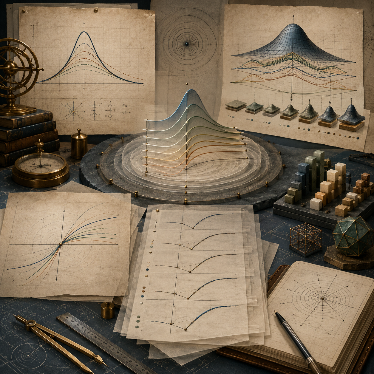
Taylor and Maclaurin series are often introduced as formulas, but their modeling importance is deeper. They show how a function can be approximated by successively richer polynomial terms near a chosen center. The first term anchors the value. The next term describes local change. The second-order term captures curvature. Higher-order terms add increasingly refined nonlinear structure. The remainder records what the approximation leaves out.
Why Taylor and Maclaurin Series Matter
Taylor and Maclaurin series matter because many models are too complex to interpret directly but can be understood locally. A nonlinear response curve may be difficult to explain in its full form. A dynamic system may be easier to analyze near equilibrium. A cost, risk, growth, or feedback function may be approximated around a baseline scenario. Taylor series provide a disciplined way to build those approximations from derivatives.
The basic Taylor idea is that a function near \(a\) may be represented by a polynomial built from its derivatives at \(a\):
f(x)\approx f(a)+f'(a)(x-a)+\frac{f”(a)}{2!}(x-a)^2+\frac{f”'(a)}{3!}(x-a)^3+\cdots
\]
Interpretation: Local function behavior is approximated by value, slope, curvature, and higher-order derivative information at the center.
This matters for modeling because it makes approximation transparent. Instead of simply replacing a nonlinear function with a simplified expression, the Taylor structure shows what information is retained and what is omitted. A first-order model keeps value and slope. A second-order model adds curvature. Higher-order models add more local nonlinear structure.
| Modeling need | Taylor-series role | Interpretive caution |
|---|---|---|
| Linearize a nonlinear model | Use the first derivative near a reference state. | Linearization may fail far from the center. |
| Capture curvature | Add second-order terms. | Curvature is still local unless global structure is known. |
| Approximate difficult functions | Use finite Taylor polynomials. | Truncation error must be addressed. |
| Analyze equilibrium behavior | Approximate dynamics near a fixed point. | Local stability may not imply global stability. |
| Propagate uncertainty | Approximate how input variation affects output. | Large uncertainty may invalidate local approximations. |
Taylor and Maclaurin series therefore help modelers connect nonlinear functions to interpretable local structure. Their value is not only computational but explanatory.
What Is a Taylor Series?
A Taylor series centered at \(a\) represents a function as an infinite polynomial whose coefficients come from derivatives at the center:
f(x)=\sum_{n=0}^{\infty}\frac{f^{(n)}(a)}{n!}(x-a)^n
\]
Interpretation: A Taylor series uses the derivatives of \(f\) at \(a\) to build a power-series representation around \(a\).
The \(N\)-th Taylor polynomial is the finite truncation:
T_N(x)=\sum_{n=0}^{N}\frac{f^{(n)}(a)}{n!}(x-a)^n
\]
Interpretation: A Taylor polynomial keeps only terms up to degree \(N\), producing a finite approximation.
The center \(a\) is not a minor detail. It defines the reference state around which the function is being approximated. A Taylor polynomial centered at a system equilibrium describes behavior near that equilibrium. A Taylor polynomial centered at a baseline scenario describes behavior near that baseline. The same function may have different useful approximations depending on the center.
In modeling terms, a Taylor series is a local representation. It says: given what the function and its derivatives do at this reference point, what polynomial captures nearby behavior? The answer may be extremely useful, but it should not be treated as automatically valid everywhere.
What Is a Maclaurin Series?
A Maclaurin series is a Taylor series centered at zero. It has the form:
f(x)=\sum_{n=0}^{\infty}\frac{f^{(n)}(0)}{n!}x^n
\]
Interpretation: A Maclaurin series represents a function using derivative information at zero.
Maclaurin series are common because many standard functions have simple expansions around zero. For example:
e^x=1+x+\frac{x^2}{2!}+\frac{x^3}{3!}+\cdots
\]
Interpretation: The exponential function can be represented by a globally convergent Maclaurin series.
\sin x=x-\frac{x^3}{3!}+\frac{x^5}{5!}-\cdots
\]
Interpretation: The sine function is represented by alternating odd-power terms.
\cos x=1-\frac{x^2}{2!}+\frac{x^4}{4!}-\cdots
\]
Interpretation: The cosine function is represented by alternating even-power terms.
Maclaurin series are useful when zero is a meaningful reference point. In many systems, however, zero is not the operating condition. A population, concentration, temperature, price, load, or energy level may rarely operate near zero. In those cases, a Taylor series centered at a more meaningful baseline may be more appropriate.
Maclaurin series are therefore not automatically better than Taylor series. They are Taylor series with a particular center. The modeling question is whether that center makes sense.
Derivatives as Coefficients
The distinctive feature of Taylor series is that derivatives become coefficients. The coefficient of each power records derivative information at the center:
c_n=\frac{f^{(n)}(a)}{n!}
\]
Interpretation: The \(n\)-th coefficient is the \(n\)-th derivative at the center, scaled by \(n!\).
This gives Taylor polynomials strong interpretive value. The constant term gives the value of the function at the center. The linear term gives local slope. The second-order term gives curvature. Higher-order terms encode increasingly subtle local behavior.
| Taylor term | Derivative source | Modeling interpretation |
|---|---|---|
| \(f(a)\) | Function value | Baseline system value at the reference point. |
| \(f'(a)(x-a)\) | First derivative | Local marginal change, sensitivity, or slope. |
| \(\frac{f”(a)}{2!}(x-a)^2\) | Second derivative | Curvature, acceleration, convexity, or diminishing response. |
| \(\frac{f”'(a)}{3!}(x-a)^3\) | Third derivative | Asymmetry, inflection behavior, or nonlinear skew. |
| Higher-order terms | Higher derivatives | Fine-grained nonlinear structure near the center. |
Because derivatives have modeling meaning, Taylor coefficients do too. The series is not just a computational device; it is a structured explanation of local behavior.
First-Order Approximation and Linearization
The first-order Taylor approximation keeps only the value and slope terms:
f(x)\approx f(a)+f'(a)(x-a)
\]
Interpretation: Near \(a\), the function is approximated by its tangent line.
This is one of the most important tools in applied modeling. It turns nonlinear behavior into a local linear relationship. That can make a model easier to analyze, communicate, compute, and compare. In dynamic systems, linearization near equilibrium helps determine local stability. In economics, it supports marginal analysis. In engineering, it approximates response near an operating point. In uncertainty analysis, it estimates how small input changes affect output.
First-order approximation is useful because it is simple. It is also risky because it ignores curvature and higher-order structure. If the function bends sharply, if the input change is large, or if the system is near a threshold, the tangent-line approximation may be misleading.
| Use case | First-order approximation helps by | Risk |
|---|---|---|
| Local sensitivity | Estimating output response to small input changes. | Sensitivity may change away from the center. |
| Equilibrium analysis | Approximating dynamics near a fixed point. | Large disturbances may leave the local region. |
| Policy threshold analysis | Estimating near-baseline effects. | Nonlinear thresholds may be missed. |
| Numerical methods | Replacing a function by a local tangent model. | Step size may be too large for linear validity. |
Linearization is therefore a disciplined local approximation, not a claim that the world is linear.
In higher-dimensional models, the same idea becomes local linearization by gradients or Jacobians. A scalar function \(f(x_1,\ldots,x_m)\) is approximated by its value and gradient near a point. A vector-valued system is approximated by its Jacobian matrix. This is why Taylor expansion sits behind sensitivity analysis, state-space linearization, local stability analysis, and many numerical solvers: it converts local nonlinear behavior into a structured first-order map whose limits can be examined.
Second-Order Approximation and Curvature
The second-order Taylor approximation adds curvature:
f(x)\approx f(a)+f'(a)(x-a)+\frac{f”(a)}{2}(x-a)^2
\]
Interpretation: A second-order approximation captures baseline value, local slope, and curvature.
Second-order terms matter when response is not adequately described by a tangent line. Curvature can indicate acceleration, saturation, convexity, concavity, diminishing returns, increasing risk, or local stability structure. In optimization, second-order information helps classify local minima and maxima. In dynamic systems, curvature helps reveal nonlinear response near equilibria.
The sign of the second derivative is often important:
f”(a)>0\quad\text{suggests local convexity},\qquad f”(a)<0\quad\text{suggests local concavity}
\]
Interpretation: The second derivative describes local bending behavior near the center.
Second-order approximation is still local. It may be much better than a linear approximation near the center but still unreliable far away. The modeler must still ask how large the displacement is, what error is acceptable, and whether higher-order terms matter.
For functions of several variables, second-order information is carried by the Hessian matrix. The Hessian records how sensitivities themselves change with respect to inputs. In optimization and stability analysis, this distinction matters: a gradient can show the direction of local change, while the Hessian can reveal local curvature, interaction among variables, and whether the neighborhood behaves like a valley, ridge, saddle, or flat region. In systems language, curvature often marks whether a small stress remains proportional or begins to amplify.
Higher-Order Terms and Nonlinear Structure
Higher-order Taylor terms refine local representation. They can capture asymmetry, inflection, oscillation, rapid growth, saturation, or more complicated nonlinear behavior. The \(N\)-th Taylor polynomial is:
T_N(x)=f(a)+f'(a)(x-a)+\frac{f”(a)}{2!}(x-a)^2+\cdots+\frac{f^{(N)}(a)}{N!}(x-a)^N
\]
Interpretation: Increasing \(N\) adds higher-order derivative information to the local polynomial approximation.
Adding more terms can improve approximation, but it does not automatically improve modeling judgment. More terms can increase computational burden, produce unstable behavior outside the valid interval, create false confidence, or obscure interpretation. A higher-order polynomial may fit local behavior well but behave strangely outside the region where the approximation is justified.
In systems modeling, higher-order terms are especially useful when the modeler needs to represent nonlinear response but still wants a structured approximation. They are common in perturbation methods, asymptotic analysis, local nonlinear dynamics, numerical solvers, and sensitivity expansions. They are less useful when the underlying system has discontinuities, thresholds, regime shifts, or abrupt shocks that cannot be captured by smooth local derivatives.
Remainder and Error
The difference between the function and the Taylor polynomial is the remainder:
R_N(x)=f(x)-T_N(x)
\]
Interpretation: The remainder records the error introduced by truncating the Taylor series after degree \(N\).
The Taylor formula with remainder is:
f(x)=T_N(x)+R_N(x)
\]
Interpretation: A Taylor polynomial plus its remainder equals the original function when the formula applies.
One common form is the Lagrange remainder:
R_N(x)=\frac{f^{(N+1)}(\xi)}{(N+1)!}(x-a)^{N+1}
\]
Interpretation: For some \(\xi\) between \(a\) and \(x\), the next derivative controls the truncation error.
Remainder logic is essential for responsible modeling. A finite Taylor polynomial can always be computed if the derivatives are available. But computation is not the same as accuracy. The modeler must ask how large the omitted terms may be, whether an error bound is available, and whether the approximation is sufficient for the decision or explanation being made.
| Approximation claim | Required error question |
|---|---|
| First-order approximation is enough. | How large is the omitted curvature and higher-order structure? |
| Second-order approximation captures the behavior. | Are third and higher terms small over the use interval? |
| The polynomial matches the function near the center. | How far from the center was this checked? |
| The numerical result is stable. | Was error bounded, or merely observed to be small? |
Without remainder logic, Taylor approximation becomes a guess that happens to use calculus notation.
Big-O notation gives another compact way to describe omitted structure. A first-order approximation may be written as \(f(a+h)=f(a)+f'(a)h+O(h^2)\), meaning the omitted terms are bounded in size like a constant multiple of \(h^2\) near the center under appropriate assumptions. A second-order approximation may leave an \(O(h^3)\) remainder. This notation is useful because it connects approximation order to displacement size: halving the displacement can reduce the leading omitted term dramatically, but only within a region where the assumptions behind the expansion remain valid.
Convergence Versus Useful Approximation
Taylor and Maclaurin series raise two different questions. First, does the infinite series converge? Second, does a finite truncation provide a useful approximation for the modeling purpose? These questions are related but not identical.
An infinite Taylor series may converge only within a certain radius. It may converge slowly. It may converge but require many terms for useful accuracy. In some pathological cases, a function may have derivatives of all orders, yet the Taylor series may not represent the function away from the center.
| Question | Meaning | Modeling implication |
|---|---|---|
| Does the series converge? | The infinite polynomial approaches a finite value. | The representation may be mathematically meaningful in a domain. |
| Does it converge to the function? | The series equals the target function in that domain. | The representation is analytically valid. |
| Is the truncation accurate enough? | The finite polynomial is close enough for the purpose. | The approximation may support computation or interpretation. |
| Is the use domain local enough? | The evaluation points remain near the center. | The model does not overextend local structure. |
A finite Taylor approximation can be useful even when the infinite series is not being used explicitly. But the modeler should not confuse practical usefulness with unlimited validity. Useful local approximation still requires scope and error discipline.
This distinction is especially important in perturbation and asymptotic methods. Some expansions are designed to be useful for small parameters even when they are not convergent power series in the ordinary sense. Other expansions converge but do so too slowly to be computationally efficient at the point of use. The practical question is therefore layered: whether the series converges, whether it converges to the intended function, whether the finite truncation is accurate enough, and whether the approximation remains meaningful for the system state being modeled.
Common Series in Modeling
Several Taylor and Maclaurin series appear frequently in modeling and computation. They are useful because they approximate standard functions that arise in growth, oscillation, saturation, probability, physics, finance, and numerical methods.
| Function | Maclaurin series | Common modeling use |
|---|---|---|
| \(e^x\) | \(\sum_{n=0}^{\infty}\frac{x^n}{n!}\) | Growth, decay, compounding, probability, differential equations. |
| \(\sin x\) | \(\sum_{n=0}^{\infty}(-1)^n\frac{x^{2n+1}}{(2n+1)!}\) | Oscillation, waves, cycles, rotations, periodic forcing. |
| \(\cos x\) | \(\sum_{n=0}^{\infty}(-1)^n\frac{x^{2n}}{(2n)!}\) | Oscillation, equilibrium, wave models, harmonic motion. |
| \(\ln(1+x)\) | \(\sum_{n=1}^{\infty}(-1)^{n+1}\frac{x^n}{n}\) | Elasticity, proportional change, information measures, approximations. |
| \(\frac{1}{1-x}\) | \(\sum_{n=0}^{\infty}x^n\) | Feedback multipliers, discounting, repeated proportional effects. |
Each series has its own convergence behavior and interpretation. Some converge for all real \(x\). Others have limited intervals. The modeling value of a series depends not only on the formula but also on where it is used.
Systems Modeling Interpretation
In systems modeling, Taylor and Maclaurin series provide a bridge from formal calculus to practical interpretation. They help explain why a nonlinear function may behave almost linearly near a point, why curvature matters, why small perturbations can be approximated, and why large deviations may require a different model.
Consider a system output \(y=f(x)\) near a baseline \(a\). A Taylor approximation can decompose the output change into components:
\Delta y\approx f'(a)\Delta x+\frac{f”(a)}{2}(\Delta x)^2+\cdots
\]
Interpretation: Output change is decomposed into first-order sensitivity, curvature, and higher-order effects.
This supports several modeling habits. The first-order term helps explain local sensitivity. The second-order term shows whether response bends. Higher-order terms warn that nonlinear structure may matter. The omitted remainder reminds the modeler that approximation has limits.
For dynamic systems, Taylor expansion near an equilibrium can support local stability analysis. For environmental systems, it can approximate response around a baseline climate, load, or concentration. For economic systems, it can approximate cost, utility, growth, or risk functions. For infrastructure systems, it can approximate congestion near a capacity threshold, though thresholds may also expose the limits of smooth approximation.
The central interpretation is local. Taylor series are powerful when the center, domain, and error are respected. They are misleading when a local polynomial is treated as a global description of a complex system.
Multivariable Taylor Expansions, Jacobians, and Hessians
Systems models rarely depend on one variable alone. They often involve interacting inputs: temperature and humidity, price and demand, traffic and capacity, emissions and removals, population and exposure, state variables and control variables. Taylor expansion extends naturally to these settings by replacing ordinary derivatives with gradients, Jacobians, and Hessians.
For a scalar function of several variables, the first-order approximation around a point \(a\) can be written using a displacement vector \(h=x-a\):
f(a+h)\approx f(a)+\nabla f(a)^T h
\]
Interpretation: The gradient gives the local sensitivity of the output to small changes in all input directions.
The second-order approximation adds curvature through the Hessian matrix:
f(a+h)\approx f(a)+\nabla f(a)^T h+\frac{1}{2}h^T H_f(a)h
\]
Interpretation: The Hessian describes how curvature and input interactions shape the local response.
For vector-valued systems, the Jacobian plays the first-order role. If \(F:\mathbb{R}^m\to\mathbb{R}^k\), then near \(a\):
F(a+h)\approx F(a)+J_F(a)h
\]
Interpretation: The Jacobian maps small input displacements into approximate output displacements.
This is the mathematical engine behind local sensitivity analysis, linearized dynamics, uncertainty propagation, and many control and optimization methods. The approximation is powerful because it compresses local system behavior into derivative objects. It is limited because those derivative objects describe a neighborhood, not the whole landscape.
| Object | Mathematical role | Systems interpretation |
|---|---|---|
| Gradient | First derivatives of a scalar output. | Local sensitivity to each input direction. |
| Jacobian | First derivatives of a vector-valued map. | Local input-output structure for multi-state systems. |
| Hessian | Second derivatives of a scalar output. | Curvature, interaction, convexity, saddle behavior, or nonlinear amplification. |
| Displacement vector | Movement away from the center. | Scenario change, perturbation, shock, or local deviation. |
Multivariable Taylor expansion helps make local complexity interpretable. It also makes the boundary of interpretation clearer: as the displacement grows, omitted terms and nonlinear interactions may dominate the derivative information used at the center.
Taylor Expansions in Dynamical Systems
Dynamic systems often depend on local behavior near equilibrium. Suppose a continuous-time system is written as:
\frac{dx}{dt}=F(x)
\]
Interpretation: The state changes according to a vector field \(F\).
If \(x^\*\) is an equilibrium, then \(F(x^\*)=0\). Near that equilibrium, the first-order Taylor expansion gives:
F(x)\approx J_F(x^\*)(x-x^\*)
\]
Interpretation: The Jacobian at the equilibrium describes the local linearized dynamics.
This linearized system can reveal whether nearby trajectories tend to return toward equilibrium, move away, oscillate, or respond differently across directions. Eigenvalues of the Jacobian often become indicators of local stability, damping, growth, rotation, or saddle behavior. The Taylor expansion does not solve the full nonlinear system, but it exposes the local mechanism that governs small disturbances.
Discrete-time systems use a similar idea. If \(x_{n+1}=G(x_n)\), then near a fixed point \(x^\*\):
x_{n+1}-x^\*\approx J_G(x^\*)(x_n-x^\*)
\]
Interpretation: The Jacobian of the update rule approximates how small deviations evolve from one step to the next.
This is why Taylor series belong in systems modeling rather than only in a calculus chapter. They connect local derivative information to stability, feedback, sensitivity, numerical integration, and the interpretation of equilibrium. The same warning remains: local stability is not global stability. A system may behave predictably near a fixed point and very differently after a large shock or outside the neighborhood where the expansion is valid.
Scaling, Step Size, and Numerical Stability
Taylor approximations also shape numerical methods. A one-step numerical method often assumes that a function behaves predictably over a small interval. The smaller the step, the more plausible the local approximation usually becomes; the larger the step, the more the omitted terms can matter.
For a small displacement \(h\), Taylor logic gives:
f(a+h)=f(a)+f'(a)h+\frac{f”(a)}{2}h^2+R_2(a+h)
\]
Interpretation: Step-size choice controls how much omitted curvature and higher-order behavior can enter the approximation.
Numerical methods use this structure in different ways. Euler’s method keeps first-order information. Higher-order Runge-Kutta methods are designed to capture more local structure without requiring explicit high derivatives. Newton’s method uses first derivative information to approximate roots locally. Optimization methods may use gradients, Hessians, or approximations to Hessians to move through a response surface.
| Numerical setting | Taylor-series connection | Review question |
|---|---|---|
| Euler stepping | First-order local approximation. | Is the step size small enough for the omitted terms? |
| Runge-Kutta methods | Higher-order local accuracy through staged evaluations. | Was local error controlled across the integration interval? |
| Newton iteration | Local linear approximation to solve \(f(x)=0\). | Is the starting point close enough for convergence? |
| Quadratic optimization | Second-order approximation of objective behavior. | Is the Hessian reliable and well-conditioned? |
| Surrogate modeling | Polynomial approximation of a complex response. | Is the approximation validated outside the calibration neighborhood? |
Scaling matters as much as step size. If variables have very different units or magnitudes, a Taylor approximation may be numerically awkward even when it is mathematically valid. Centering, nondimensionalization, and careful scaling can make derivative coefficients more interpretable and reduce numerical instability. A model that records its expansion center but not its scaling still leaves part of the approximation logic hidden.
Mathematical Deepening
The formal structure of Taylor and Maclaurin series is sharper than the familiar approximation formulas suggest. These are derivative-built power series whose meaning depends on differentiability, coefficient construction, convergence, equality to the target function, and remainder behavior. A Taylor polynomial is not merely a fitted curve. It is a structured local approximation generated from derivative information, and its credibility depends on how that local structure is used.
Formal Structure
Taylor Series
A Taylor series centered at \(a\) uses derivatives at \(a\) to construct a power series in \(x-a\).
Maclaurin Series
A Maclaurin series is a Taylor series centered at zero.
Taylor Polynomial
The \(N\)-th Taylor polynomial keeps terms through degree \(N\).
Remainder
The remainder records the difference between the function and the finite Taylor polynomial.
Representation Conditions
Differentiability
Derivative-based coefficients require the relevant derivatives to exist at the expansion center.
Convergence
The infinite series must converge in the region where it is used.
Analytic Equality
The Taylor series must converge to the function, not merely converge to some value.
Error Control
Finite truncations require remainder estimates or validity warnings.
Counterexamples and Warnings
Smooth Does Not Always Mean Analytic
A function may have derivatives of all orders without being represented by its Taylor series away from the center.
Local Does Not Mean Global
A Taylor polynomial may work near the center but fail under large displacement.
Truncation Is Not Equality
A finite Taylor polynomial omits higher-order terms that may matter.
Thresholds Break Smooth Logic
Discontinuities, shocks, and regime shifts may not be captured by smooth local expansion.
Advanced Modeling Implications
State the Center
Every Taylor approximation should identify the expansion center and why it was chosen.
State the Order
The truncation order should be reported so readers know which derivative information was retained.
State the Error Logic
Approximations should include a remainder estimate, tolerance, or limitation statement.
State the Use Domain
The local region where the approximation is intended to hold should be made explicit.
Examples from Systems Modeling
Taylor and Maclaurin series appear whenever systems models approximate nonlinear relationships using local derivative information. These examples show how the method supports interpretation while requiring scope discipline.
Local Stability Near Equilibrium
First-order Taylor expansion helps analyze how a dynamic system responds to small disturbances near a fixed point.
Nonlinear Cost Curves
Second-order approximation can show whether marginal cost increases, decreases, or bends near a baseline output level.
Climate Sensitivity Approximation
Local expansions can approximate response around a baseline forcing level while warning against overextension.
Uncertainty Propagation
Taylor terms can estimate how input uncertainty affects nonlinear output behavior near a reference scenario.
Numerical Solvers
Taylor logic underlies many numerical methods that step through local approximations of change.
Feedback Linearization
Nonlinear feedback relationships can sometimes be approximated locally to study near-baseline response.
Across these cases, Taylor series clarify local structure. They do not eliminate the need to check domain, error, and nonlinear behavior beyond the expansion center.
Computation and Reproducible Workflows
Computational Taylor workflows should record the target function, expansion center, derivative or coefficient rule, approximation order, evaluation points, finite approximation, reference value when available, error estimate, convergence or domain warning, and interpretation. They should separate the full function from the Taylor polynomial and the Taylor polynomial from its modeling claim.
Good workflows evaluate multiple truncation orders and multiple distances from the center. They show how error changes as terms are added. They warn when the evaluation point is outside the intended local region. They store outputs in CSV and JSON formats so approximation claims can be reviewed later.
For multidimensional models, the workflow should also record the variables included in the expansion, the scaling of each variable, the gradient or Jacobian source, and any Hessian or curvature assumptions. If derivatives are computed numerically, the finite-difference step, automatic-differentiation tool, or symbolic source should be recorded. Taylor approximations are often only as credible as the derivative pipeline that produced their coefficients.
Python Workflow: Taylor Approximation Audit
The Python workflow below compares finite Taylor approximations for \(e^x\), records approximation error, and writes auditable outputs.
from __future__ import annotations

from dataclasses import dataclass, asdict
from pathlib import Path
import csv
import json
import math


@dataclass(frozen=True)
class TaylorAudit:
    function_name: str
    center: float
    x_value: float
    order: int
    approximation: float
    reference_value: float
    absolute_error: float
    warning: str


def taylor_exp_maclaurin(x: float, order: int) -> float:
    return sum((x ** n) / math.factorial(n) for n in range(order + 1))


def audit_exp(x: float, order: int) -> TaylorAudit:
    approximation = taylor_exp_maclaurin(x, order)
    reference = math.exp(x)
    return TaylorAudit(
        function_name="exp(x)",
        center=0.0,
        x_value=x,
        order=order,
        approximation=approximation,
        reference_value=reference,
        absolute_error=abs(reference - approximation),
        warning="" if abs(x) <= 2 else "Evaluation is far from the Maclaurin center; review truncation error carefully."
    )


records = [
    audit_exp(0.5, 2),
    audit_exp(0.5, 5),
    audit_exp(1.0, 5),
    audit_exp(1.0, 10),
    audit_exp(3.0, 10)
]

output_dir = Path("outputs")
(output_dir / "tables").mkdir(parents=True, exist_ok=True)
(output_dir / "json").mkdir(parents=True, exist_ok=True)

with (output_dir / "tables" / "taylor_exp_approximation_audit.csv").open("w", newline="", encoding="utf-8") as handle:
    writer = csv.DictWriter(handle, fieldnames=asdict(records[0]).keys())
    writer.writeheader()
    for record in records:
        writer.writerow(asdict(record))

(output_dir / "json" / "taylor_exp_approximation_audit.json").write_text(
    json.dumps([asdict(record) for record in records], indent=2),
    encoding="utf-8"
)

print("Wrote Taylor approximation audit.")
This workflow keeps the approximation, reference value, error, order, center, and warning separate.
R Workflow: Local Approximation Diagnostics
The R workflow below compares Maclaurin approximations of \(e^x\) at different orders and evaluation points.
# Taylor and Maclaurin Series in Modeling
# Base R workflow for local approximation diagnostics.

taylor_exp_maclaurin <- function(x, order) {
  n <- 0:order
  sum((x^n) / factorial(n))
}

audit_exp <- function(x, order) {
  approximation <- taylor_exp_maclaurin(x, order)
  reference_value <- exp(x)

  data.frame(
    function_name = "exp(x)",
    center = 0,
    x_value = x,
    order = order,
    approximation = approximation,
    reference_value = reference_value,
    absolute_error = abs(reference_value - approximation),
    warning = ifelse(abs(x) <= 2, "", "Evaluation is far from the Maclaurin center; review truncation error carefully.")
  )
}

cases <- rbind(
  audit_exp(0.5, 2),
  audit_exp(0.5, 5),
  audit_exp(1.0, 5),
  audit_exp(1.0, 10),
  audit_exp(3.0, 10)
)

dir.create("outputs/tables", recursive = TRUE, showWarnings = FALSE)
write.csv(cases, "outputs/tables/r_taylor_exp_approximation_audit.csv", row.names = FALSE)

print(cases)
This workflow supports a simple audit habit: compare approximation error across both order and distance from the center.
Haskell Workflow: Typed Taylor Records
Haskell can represent Taylor approximation records with explicit types for center, order, approximation, error, and warning.
module Main where

newtype Center = Center Double deriving (Show)
newtype XValue = XValue Double deriving (Show)
newtype Order = Order Int deriving (Show)
newtype Approximation = Approximation Double deriving (Show)
newtype ReferenceValue = ReferenceValue Double deriving (Show)
newtype AbsoluteError = AbsoluteError Double deriving (Show)

data TaylorAudit = TaylorAudit
  { functionName :: String
  , center :: Center
  , xValue :: XValue
  , order :: Order
  , approximation :: Approximation
  , referenceValue :: ReferenceValue
  , absoluteError :: AbsoluteError
  , warning :: String
  } deriving (Show)

factorial :: Int -> Double
factorial n = product [1.0..fromIntegral n]

taylorExpMaclaurin :: Double -> Int -> Double
taylorExpMaclaurin x orderValue =
  sum [(x ** fromIntegral n) / factorial n | n <- [0..orderValue]]

auditExp :: Double -> Int -> TaylorAudit
auditExp x orderValue =
  let approximationValue = taylorExpMaclaurin x orderValue
      reference = exp x
      warningText = if abs x <= 2 then "" else "Evaluation is far from the Maclaurin center; review truncation error carefully."
  in TaylorAudit
      { functionName = "exp(x)"
      , center = Center 0.0
      , xValue = XValue x
      , order = Order orderValue
      , approximation = Approximation approximationValue
      , referenceValue = ReferenceValue reference
      , absoluteError = AbsoluteError (abs (reference - approximationValue))
      , warning = warningText
      }

main :: IO ()
main = do
  print (auditExp 0.5 2)
  print (auditExp 0.5 5)
  print (auditExp 1.0 10)
  print (auditExp 3.0 10)
The typed structure helps prevent approximation order, reference value, and error from being collapsed into a single uninterpreted number.
SQL Workflow: Taylor Approximation Assumption Registry
SQL can document the assumptions behind Taylor and Maclaurin approximations when they support dashboards, reports, governance workflows, or reproducible modeling systems.
CREATE TABLE taylor_approximation_assumption_registry (
    assumption_key TEXT PRIMARY KEY,
    assumption_name TEXT NOT NULL,
    mathematical_role TEXT NOT NULL,
    systems_modeling_role TEXT NOT NULL,
    review_warning TEXT NOT NULL
);

INSERT INTO taylor_approximation_assumption_registry VALUES
(
  'expansion_center',
  'Expansion center',
  'Defines the point where derivative information is taken.',
  'Identifies the local reference state for interpretation.',
  'A Taylor approximation should not be interpreted without knowing its center.'
);

INSERT INTO taylor_approximation_assumption_registry VALUES
(
  'approximation_order',
  'Approximation order',
  'Records the highest retained polynomial degree.',
  'Shows which derivative information was included or omitted.',
  'A first-order approximation may miss important curvature or nonlinear response.'
);

INSERT INTO taylor_approximation_assumption_registry VALUES
(
  'derivative_provenance',
  'Derivative provenance',
  'Documents how derivative values or coefficients were obtained.',
  'Separates symbolic, numerical, estimated, and assumed derivative information.',
  'Derivative coefficients without provenance are difficult to audit.'
);

INSERT INTO taylor_approximation_assumption_registry VALUES
(
  'remainder_logic',
  'Remainder logic',
  'Describes the omitted terms or error estimate.',
  'Supports responsible interpretation of finite Taylor polynomials.',
  'A Taylor polynomial should not be trusted without error or validity review.'
);

INSERT INTO taylor_approximation_assumption_registry VALUES
(
  'local_validity',
  'Local validity',
  'Defines the region where the approximation is intended to apply.',
  'Prevents local polynomial behavior from being treated as global system truth.',
  'Large shocks, thresholds, and regime changes may invalidate local approximation.'
);

SELECT
    assumption_name,
    mathematical_role,
    systems_modeling_role,
    review_warning
FROM taylor_approximation_assumption_registry
ORDER BY assumption_key;
This registry keeps Taylor approximation interpretation tied to center, order, derivative provenance, remainder logic, and local validity.
GitHub Repository
The companion repository for this article is designed as a reproducible mathematical-modeling workspace. It supports Taylor approximation audits, Maclaurin series examples, derivative-based coefficient records, truncation-error diagnostics, local-validity review, SQL assumption registries, generated outputs, advanced mathematical audit reports, and reusable calculator scripts.
Complete Code Repository
Companion article folder with Python, R, Julia, SQL, Haskell, C, C++, Fortran, Rust, Go, notebooks, documentation, synthetic teaching data, generated outputs, schemas, Canvas-ready workflow artifacts, and reusable calculator scripts for Taylor series, Maclaurin series, local approximation, linearization, curvature, truncation error, derivative-based coefficients, multivariable Taylor expansion, Jacobian and Hessian diagnostics, step-size logic, numerical approximation, and responsible mathematical modeling.
Interpretive Limits and Responsible Use
Taylor and Maclaurin series are powerful because they make local approximation systematic. They are also easy to overextend. A Taylor polynomial may be accurate near the center and poor farther away. A first-order approximation may miss curvature. A second-order approximation may miss thresholds or asymmetry. A smooth local expansion may fail to describe shocks, discontinuities, regime shifts, or boundary effects.
Responsible use requires several checks. State the expansion center. State the approximation order. Explain how derivatives or coefficients were obtained. Report the evaluation region. Estimate or discuss the remainder. Distinguish convergence of the series from accuracy of the finite polynomial. Avoid treating local approximation as global explanation. Clarify what system behavior is preserved and what is lost.
The central modeling question is not only “Can I write down a Taylor series?” It is “What does this approximation preserve, what does it omit, how large is the omitted part, and how far from the center can the interpretation be trusted?”
Related Articles
- Calculus for Systems Modeling
- Power Series and Functional Representation
- Convergence Tests and the Discipline of Infinite Approximation
- Approximation Error, Truncation, and Local Validity
- Differentiability and Local Behavior
- Second Derivatives, Curvature, and Acceleration
- Functions of Several Variables
- Numerical Methods for Systems Modeling
- Scientific Computing for Systems Modeling
- Model Governance and Accountability
Further Reading
- Abbott, S. (2015) Understanding Analysis. 2nd edn. New York: Springer. Available at: https://link.springer.com/book/10.1007/978-1-4939-2712-8.
- Apostol, T.M. (1967) Calculus, Volume 1: One-Variable Calculus, with an Introduction to Linear Algebra. 2nd edn. New York: Wiley. Available at: https://www.wiley.com/en-us/Calculus%2C+Volume+1%2C+2nd+Edition-p-9780471000051.
- Apostol, T.M. (1969) Calculus, Volume 2: Multi-Variable Calculus and Linear Algebra, with Applications to Differential Equations and Probability. 2nd edn. New York: Wiley. Available at: https://www.wiley.com/en-us/Calculus%2C+Volume+2%2C+2nd+Edition-p-9780471000075.
- Burden, R.L., Faires, J.D. and Burden, A.M. (2015) Numerical Analysis. 10th edn. Boston, MA: Cengage Learning. Available at: https://www.cengage.com/c/numerical-analysis-10e-burden/.
- Courant, R. and John, F. (1999) Introduction to Calculus and Analysis, Volume I. Berlin: Springer. Available at: https://link.springer.com/book/10.1007/978-3-642-58604-0.
- Hairer, E., Nørsett, S.P. and Wanner, G. (1993) Solving Ordinary Differential Equations I: Nonstiff Problems. 2nd edn. Berlin: Springer. Available at: https://link.springer.com/book/10.1007/978-3-540-78862-1.
- Higham, N.J. (2002) Accuracy and Stability of Numerical Algorithms. 2nd edn. Philadelphia, PA: Society for Industrial and Applied Mathematics. Available at: https://epubs.siam.org/doi/book/10.1137/1.9780898718027.
- Knopp, K. (1990) Theory and Application of Infinite Series. New York: Dover Publications. Available at: https://store.doverpublications.com/products/9780486661650.
- National Institute of Standards and Technology (n.d.) DLMF: Chapter 1, Algebraic and Analytic Methods. NIST Digital Library of Mathematical Functions. Available at: https://dlmf.nist.gov/1.
- National Institute of Standards and Technology (n.d.) DLMF: Chapter 2, Asymptotic Approximations. NIST Digital Library of Mathematical Functions. Available at: https://dlmf.nist.gov/2.
- National Institute of Standards and Technology (n.d.) DLMF: Chapter 4, Elementary Functions. NIST Digital Library of Mathematical Functions. Available at: https://dlmf.nist.gov/4.
- OpenStax (2016) Calculus Volume 2. Houston, TX: OpenStax, Rice University. Available at: https://openstax.org/details/books/calculus-volume-2.
- Rudin, W. (1976) Principles of Mathematical Analysis. 3rd edn. New York: McGraw-Hill. Available at: https://www.mheducation.com/highered/product/principles-mathematical-analysis-rudin/M9780070542358.html.
- Spivak, M. (2008) Calculus. 4th edn. Houston, TX: Publish or Perish. Available at: https://www.publishorperish.com/Calculus.
- Stein, E.M. and Shakarchi, R. (2003) Complex Analysis. Princeton, NJ: Princeton University Press. Available at: https://press.princeton.edu/books/hardcover/9780691113852/complex-analysis.
- Süli, E. and Mayers, D.F. (2003) An Introduction to Numerical Analysis. Cambridge: Cambridge University Press. Available at: https://www.cambridge.org/highereducation/books/an-introduction-to-numerical-analysis/6A91A47287B6F4C5C51D7B4E1207DDE2.
- Trefethen, L.N. (2013) Approximation Theory and Approximation Practice. Philadelphia, PA: Society for Industrial and Applied Mathematics. Available at: https://epubs.siam.org/doi/book/10.1137/1.9781611972405.
- Massachusetts Institute of Technology OpenCourseWare (2010) Single Variable Calculus. Cambridge, MA: MIT OpenCourseWare. Available at: https://ocw.mit.edu/courses/18-01sc-single-variable-calculus-fall-2010/.
- Massachusetts Institute of Technology OpenCourseWare (2011) Differential Equations. Cambridge, MA: MIT OpenCourseWare. Available at: https://ocw.mit.edu/courses/18-03sc-differential-equations-fall-2011/.
- Massachusetts Institute of Technology OpenCourseWare (2010) Multivariable Calculus. Cambridge, MA: MIT OpenCourseWare. Available at: https://ocw.mit.edu/courses/18-02sc-multivariable-calculus-fall-2010/.
- SciPy Developers (n.d.) Special Functions: scipy.special. SciPy Documentation. Available at: https://docs.scipy.org/doc/scipy/reference/special.html.
- NumPy Developers (n.d.) Polynomials. NumPy Documentation. Available at: https://numpy.org/doc/stable/reference/routines.polynomials.html.
References
- Abbott, S. (2015) Understanding Analysis. 2nd edn. New York: Springer. Available at: https://link.springer.com/book/10.1007/978-1-4939-2712-8.
- Apostol, T.M. (1967) Calculus, Volume 1: One-Variable Calculus, with an Introduction to Linear Algebra. 2nd edn. New York: Wiley. Available at: https://www.wiley.com/en-us/Calculus%2C+Volume+1%2C+2nd+Edition-p-9780471000051.
- Apostol, T.M. (1969) Calculus, Volume 2: Multi-Variable Calculus and Linear Algebra, with Applications to Differential Equations and Probability. 2nd edn. New York: Wiley. Available at: https://www.wiley.com/en-us/Calculus%2C+Volume+2%2C+2nd+Edition-p-9780471000075.
- Burden, R.L., Faires, J.D. and Burden, A.M. (2015) Numerical Analysis. 10th edn. Boston, MA: Cengage Learning. Available at: https://www.cengage.com/c/numerical-analysis-10e-burden/.
- Courant, R. and John, F. (1999) Introduction to Calculus and Analysis, Volume I. Berlin: Springer. Available at: https://link.springer.com/book/10.1007/978-3-642-58604-0.
- Hairer, E., Nørsett, S.P. and Wanner, G. (1993) Solving Ordinary Differential Equations I: Nonstiff Problems. 2nd edn. Berlin: Springer. Available at: https://link.springer.com/book/10.1007/978-3-540-78862-1.
- Higham, N.J. (2002) Accuracy and Stability of Numerical Algorithms. 2nd edn. Philadelphia, PA: Society for Industrial and Applied Mathematics. Available at: https://epubs.siam.org/doi/book/10.1137/1.9780898718027.
- Knopp, K. (1990) Theory and Application of Infinite Series. New York: Dover Publications. Available at: https://store.doverpublications.com/products/9780486661650.
- National Institute of Standards and Technology (n.d.) DLMF: Chapter 1, Algebraic and Analytic Methods. NIST Digital Library of Mathematical Functions. Available at: https://dlmf.nist.gov/1.
- National Institute of Standards and Technology (n.d.) DLMF: Chapter 2, Asymptotic Approximations. NIST Digital Library of Mathematical Functions. Available at: https://dlmf.nist.gov/2.
- National Institute of Standards and Technology (n.d.) DLMF: Chapter 4, Elementary Functions. NIST Digital Library of Mathematical Functions. Available at: https://dlmf.nist.gov/4.
- OpenStax (2016) Calculus Volume 2. Houston, TX: OpenStax, Rice University. Available at: https://openstax.org/details/books/calculus-volume-2.
- Rudin, W. (1976) Principles of Mathematical Analysis. 3rd edn. New York: McGraw-Hill. Available at: https://www.mheducation.com/highered/product/principles-mathematical-analysis-rudin/M9780070542358.html.
- Spivak, M. (2008) Calculus. 4th edn. Houston, TX: Publish or Perish. Available at: https://www.publishorperish.com/Calculus.
- Stein, E.M. and Shakarchi, R. (2003) Complex Analysis. Princeton, NJ: Princeton University Press. Available at: https://press.princeton.edu/books/hardcover/9780691113852/complex-analysis.
- Süli, E. and Mayers, D.F. (2003) An Introduction to Numerical Analysis. Cambridge: Cambridge University Press. Available at: https://www.cambridge.org/highereducation/books/an-introduction-to-numerical-analysis/6A91A47287B6F4C5C51D7B4E1207DDE2.
- Trefethen, L.N. (2013) Approximation Theory and Approximation Practice. Philadelphia, PA: Society for Industrial and Applied Mathematics. Available at: https://epubs.siam.org/doi/book/10.1137/1.9781611972405.
- Massachusetts Institute of Technology OpenCourseWare (2010) Single Variable Calculus. Cambridge, MA: MIT OpenCourseWare. Available at: https://ocw.mit.edu/courses/18-01sc-single-variable-calculus-fall-2010/.
- Massachusetts Institute of Technology OpenCourseWare (2010) Multivariable Calculus. Cambridge, MA: MIT OpenCourseWare. Available at: https://ocw.mit.edu/courses/18-02sc-multivariable-calculus-fall-2010/.
- Massachusetts Institute of Technology OpenCourseWare (2011) Differential Equations. Cambridge, MA: MIT OpenCourseWare. Available at: https://ocw.mit.edu/courses/18-03sc-differential-equations-fall-2011/.
- NumPy Developers (n.d.) Polynomials. NumPy Documentation. Available at: https://numpy.org/doc/stable/reference/routines.polynomials.html.
- SciPy Developers (n.d.) Special Functions: scipy.special. SciPy Documentation. Available at: https://docs.scipy.org/doc/scipy/reference/special.html.