
Last Updated August 6, 2026
Biophysics studies life through the principles of physics: energy, entropy, force, diffusion, transport, mechanics, electrostatics, molecular structure, information, and nonequilibrium dynamics.
Living systems are made of matter, constrained by thermodynamics, driven by chemical potentials, organized by molecular interactions, and sustained by flows of energy and information. A protein folds because physical interactions make some conformations more probable than others. A membrane forms because amphiphilic molecules minimize free energy in water. A neuron fires because ion gradients, electric potentials, channels, and capacitance create excitable dynamics. A cell moves because molecular motors convert chemical energy into mechanical work. A heart beats because soft matter, fluid flow, electrophysiology, and tissue mechanics are coordinated across scales.
Biophysics does not reduce life to simple mechanics. Instead, it asks how physical law becomes biological function under conditions of complexity, noise, adaptation, regulation, and nonequilibrium organization. Biological matter is soft, wet, thermal, crowded, reactive, heterogeneous, and constantly driven. Molecules fluctuate. Cells consume energy. Membranes bend. Proteins change shape. Ion channels open and close. Motors step stochastically. Tissues remodel. Organisms maintain order by exchanging matter and energy with their surroundings. Biophysics therefore sits between molecular detail and systems behavior.
Main Library
Publications
Article Map
Physics
Related Topic
Biology
Related Topic
Chemistry
Related Topic
Astronomy
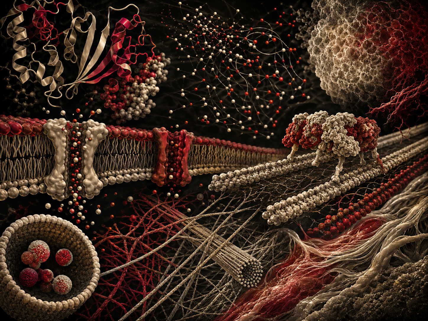
Why Biophysics Matters
Biophysics matters because living systems are physical systems that organize matter and energy in unusually complex ways. Biology cannot be fully understood from chemistry alone, nor from classical mechanics alone, nor from information theory alone. Cells and organisms integrate all of these. They transform energy, preserve structure, transmit information, respond to forces, regulate flows, and maintain internal order while remaining open to the environment.
Biophysics provides the language for explaining these processes quantitatively. It asks how molecules find each other in a crowded cell, how proteins fold, how membranes self-assemble, how ion channels generate electrical signals, how enzymes accelerate reactions, how motors walk along filaments, how DNA is packaged, how cells sense stiffness, how tissues bear load, how blood flows, and how biological networks remain robust despite noise.
The field is also central to medicine and biotechnology. Biophysical methods support structural biology, cryo-electron microscopy, x-ray crystallography, nuclear magnetic resonance, fluorescence microscopy, single-molecule force spectroscopy, patch-clamp electrophysiology, molecular dynamics simulation, drug binding studies, protein design, vaccine research, mechanobiology, bioengineering, and medical imaging. Many modern biomedical advances depend on seeing biological systems as physical systems.
For the Physics knowledge series, biophysics is important because it connects Statistical Physics and the Emergence of Macroscopic Order, Thermodynamics and the Physics of Heat, Fluid Dynamics and the Physics of Flow, Continuum Physics and Material Behavior, Electromagnetism and the Unification of Fields, Molecular Physics and the Structure of Matter, and Computational Physics and Scientific Simulation to the organization of life.
Life as Physical Organization
Living systems are organized far from thermodynamic equilibrium. A dead cell and a living cell may contain many of the same molecules, but their physical organization is different. The living cell maintains ion gradients, membrane potentials, metabolite fluxes, mechanical tension, molecular localization, reaction networks, and active transport. These structures require continuous energy dissipation.
Life therefore cannot be understood only as matter arranged in space. It must be understood as matter maintained in dynamic states by energy flow. The cell is not a static machine. It is a fluctuating, self-maintaining, chemically driven physical system.
At molecular scales, thermal fluctuations are not background noise; they are part of the operating environment. Proteins fluctuate among conformations. Ligands bind and unbind. Molecules diffuse randomly. Motors step probabilistically. Membranes undulate. DNA bends, coils, twists, and compacts. Biological function often depends on harnessing fluctuations rather than eliminating them.
This is why biophysics often emphasizes probability, free energy, stochastic processes, soft matter, and nonequilibrium dynamics. Living systems are lawful, but they are not rigid machines. They are dynamic physical systems whose reliability emerges from many noisy molecular events.
Thermal Energy and Molecular-Scale Life
At biological temperatures, thermal energy is measured by:
k_B T
\]
Interpretation: Thermal energy sets the scale of molecular fluctuations.
where \(k_B\) is Boltzmann’s constant and \(T\) is absolute temperature. Near room temperature or body temperature, \(k_B T\) is small in macroscopic units but large enough to shape molecular behavior. Many noncovalent molecular interactions have energies only a few multiples of \(k_B T\). That means thermal fluctuations can break weak interactions, shift conformational states, and drive random motion.
The Boltzmann distribution gives the relative probability of a state with energy \(E_i\):
P_i = \frac{e^{-E_i/(k_B T)}}{Z}
\]
Interpretation: Lower-energy states are more probable, but thermal fluctuations allow higher-energy states to be occupied.
where \(Z\) is the partition function:
Z = \sum_i e^{-E_i/(k_B T)}
\]
Interpretation: The partition function normalizes state probabilities.
This relation is foundational for protein conformations, ligand binding, molecular states, ion-channel gating, and thermal equilibrium models. States with lower energy are more probable, but higher-energy states can still be occupied when the energy difference is comparable to \(k_B T\).
Thermal energy makes biological systems flexible. If molecular interactions were too strong, life would be rigid and unresponsive. If they were too weak, structure would dissolve. Biological organization often occupies the delicate middle ground where interactions are stable enough to support function but weak enough to permit motion, recognition, regulation, and adaptation.
Brownian Motion and Diffusion
Brownian motion is the random motion of particles caused by collisions with surrounding molecules. In cells, Brownian motion affects proteins, metabolites, vesicles, organelles, nucleic acids, and other molecular assemblies. At small scales, random motion is not incidental; it is one of the main ways molecules explore space.
Diffusion describes the macroscopic spreading that emerges from microscopic random motion. Fick’s first law relates flux to concentration gradient:
J = -D\nabla c
\]
Interpretation: Diffusive flux moves down concentration gradients.
where \(J\) is diffusive flux, \(D\) is diffusion coefficient, and \(c\) is concentration. Fick’s second law describes how concentration changes over time:
\frac{\partial c}{\partial t} = D\nabla^2 c
\]
Interpretation: Diffusion smooths concentration differences over time.
In one dimension, the mean squared displacement for diffusion is:
\langle x^2\rangle = 2Dt
\]
Interpretation: One-dimensional diffusive spread grows linearly in time as mean squared displacement.
In three dimensions:
\langle r^2\rangle = 6Dt
\]
Interpretation: Three-dimensional mean squared displacement grows as \(6Dt\).
Diffusion is effective over short distances but slow over long distances. A small molecule may diffuse across a bacterial cell quickly, but diffusion across a large tissue would be inefficient without circulation, active transport, or structural organization. This scaling problem is one reason multicellular organisms require vascular systems, extracellular matrices, and transport networks.
Free Energy, Entropy, and Biological Order
Biological systems maintain order without violating thermodynamics because they are open systems. They exchange matter and energy with their environments. The relevant thermodynamic quantity for many biochemical processes at constant temperature and pressure is Gibbs free energy:
\Delta G = \Delta H – T\Delta S
\]
Interpretation: Gibbs free energy combines enthalpy and entropy to determine thermodynamic favorability.
where \(\Delta H\) is enthalpy change and \(\Delta S\) is entropy change. A process with:
\Delta G \lt 0
\]
Interpretation: Negative free-energy change indicates thermodynamic favorability under specified conditions.
is thermodynamically favorable under the specified conditions.
Biological order is often produced by coupling unfavorable processes to favorable ones. ATP hydrolysis, ion gradients, redox reactions, and light absorption can supply free energy to drive transport, biosynthesis, mechanical work, and signaling. Molecular motors convert chemical free energy into motion. Ion pumps use chemical energy to maintain gradients. Photosynthetic systems convert light energy into chemical and electrochemical potential.
Entropy is not the enemy of life. Entropy production is part of how living systems function. Organisms maintain local order by dissipating energy and exporting entropy to their surroundings. Biophysics therefore treats life as a nonequilibrium process, not as an exception to physical law.
Molecular Forces and Biological Structure
Biological structure is stabilized by physical interactions across multiple energy scales. Covalent bonds define molecular backbones. Hydrogen bonds, electrostatic interactions, van der Waals forces, hydrophobic effects, metal coordination, steric constraints, and solvent interactions shape folding, assembly, recognition, and dynamics.
Electrostatic interaction between two charges can be written as:
U(r) = \frac{1}{4\pi\epsilon} \frac{q_1q_2}{r}
\]
Interpretation: Coulomb energy depends on charge, separation distance, and dielectric environment.
where \(\epsilon\) is permittivity. In biological solutions, electrostatic interactions are modified by water, ions, screening, pH, local dielectric environment, and molecular geometry. The Debye length provides a scale for electrostatic screening in ionic solution.
Van der Waals interactions arise from fluctuating dipoles and short-range repulsion. Hydrogen bonds help stabilize secondary structures such as alpha helices and beta sheets. The hydrophobic effect drives nonpolar groups away from water and is central to protein folding and membrane formation.
Biological structure is therefore not determined by one force. It emerges from competing interactions, solvent effects, entropy, geometry, and thermal fluctuations. Biophysics seeks to quantify this balance.
Protein Folding and Conformational Landscapes
Proteins are polymers that fold into functional three-dimensional structures. Folding is not a simple mechanical collapse into a single rigid shape. A protein explores a conformational landscape shaped by interactions among amino acids, solvent, ions, cofactors, and other molecules.
The probability of a conformation \(i\) can be approximated by a Boltzmann factor:
P_i \propto e^{-G_i/(k_B T)}
\]
Interpretation: Protein conformations with lower free energy are more probable, but ensembles remain thermally populated.
where \(G_i\) is free energy of that conformation. The folded state is often not merely the lowest internal energy state; it is the state or ensemble that minimizes free energy under biological conditions.
Protein function often depends on conformational change. Enzymes shift between states. Receptors change shape when ligands bind. Ion channels open and close. Motor proteins cycle through mechanical states. Allosteric proteins transmit physical changes from one site to another. Disorder can also be functional; intrinsically disordered regions may enable flexible binding, signaling, and regulation.
Protein folding illustrates the central biophysical theme: biological function emerges from physical landscapes, not static structures alone.
Molecular Recognition and Binding
Molecular recognition occurs when molecules bind selectively through shape, charge, flexibility, hydrophobicity, hydrogen bonding, and dynamics. Binding is governed by free energy. For a simple ligand-receptor interaction:
R + L \rightleftharpoons RL
\]
Interpretation: Ligand binding is an equilibrium between free receptor, free ligand, and bound complex.
the dissociation constant is:
K_D = \frac{[R][L]}{[RL]}
\]
Interpretation: Lower \(K_D\) generally indicates tighter binding under the stated standard conditions.
The fraction of receptors bound is often modeled as:
\theta = \frac{[L]}{K_D+[L]}
\]
Interpretation: Binding occupancy increases with ligand concentration and reaches half-saturation at \([L]=K_D\).
Binding free energy is related to equilibrium constant:
\Delta G^\circ = RT\ln K_D
\]
Interpretation: Binding free energy is connected to the dissociation constant under standard-state conventions.
with appropriate standard-state conventions. Stronger binding corresponds to lower \(K_D\) and more favorable binding free energy.
Biological recognition is rarely just lock-and-key geometry. Many molecules bind through induced fit or conformational selection. Water displacement, entropy changes, protonation states, salt bridges, and flexibility all matter. Drug discovery, enzyme regulation, immune recognition, receptor signaling, and protein engineering all depend on understanding binding as a physical process.
Membranes as Physical Systems
Biological membranes are physical systems formed mainly by amphiphilic lipids that self-assemble in water. Their hydrophilic head groups interact with water, while hydrophobic tails avoid water, producing bilayers. Membranes are barriers, surfaces, solvents for membrane proteins, electrical capacitors, mechanical structures, and platforms for signaling.
Membrane bending energy is often modeled using curvature elasticity. A simplified Helfrich-style bending energy includes mean curvature \(H\):
E_b = \int \frac{\kappa}{2} (2H-C_0)^2 \,dA
\]
Interpretation: Membrane bending energy penalizes curvature deviations from preferred curvature.
where \(\kappa\) is bending rigidity and \(C_0\) is spontaneous curvature. This type of model helps explain vesicles, membrane tubules, budding, curvature-sensing proteins, and organelle morphology.
Membranes also have electrical properties. A membrane can be approximated as a capacitor:
C = \frac{\epsilon A}{d}
\]
Interpretation: Membrane capacitance depends on permittivity, area, and membrane thickness.
where \(A\) is area and \(d\) is membrane thickness. This capacitance is central to electrophysiology because changing membrane voltage requires moving charge.
Membranes are therefore not passive bags. They are active physical interfaces where mechanics, electrostatics, transport, chemistry, and signaling converge.
Ion Gradients and Electrochemical Potentials
Cells maintain ion gradients across membranes. These gradients store free energy and support signaling, transport, osmotic balance, motility, and metabolism. The electrochemical potential of an ion combines chemical concentration and electric potential.
For an ion of charge \(z\), the electrochemical potential can be written as:
\mu = \mu^\circ + RT\ln c + zF\phi
\]
Interpretation: Electrochemical potential combines concentration-dependent chemical energy and electrical potential energy.
where \(c\) is concentration, \(F\) is Faraday’s constant, and \(\phi\) is electric potential. At equilibrium across a membrane, the Nernst equation gives the voltage associated with an ion gradient:
E = \frac{RT}{zF} \ln \left( \frac{c_{\mathrm{out}}}{c_{\mathrm{in}}} \right)
\]
Interpretation: The Nernst equation converts an ion concentration ratio into an equilibrium voltage.
Ion gradients make cells electrically and chemically active. Sodium, potassium, calcium, chloride, and protons all play major physiological roles. Proton gradients drive ATP synthesis in mitochondria and chloroplasts. Calcium gradients support signaling. Sodium and potassium gradients support nerve impulses and secondary active transport.
Biophysics treats these gradients as stored physical work. A cell’s electrical behavior is therefore inseparable from thermodynamics, transport, and membrane structure.
Channels, Transporters, and Membrane Excitability
Ion channels allow ions to cross membranes selectively. Some channels are voltage-gated, ligand-gated, mechanically gated, or temperature-sensitive. Transporters and pumps move substances across membranes, sometimes against electrochemical gradients by using ATP, light, or coupled ion movement.
Membrane current can be modeled in a conductance form:
I = g(V-E)
\]
Interpretation: Ionic current depends on conductance and the driving force between membrane voltage and reversal potential.
where \(g\) is conductance, \(V\) is membrane potential, and \(E\) is reversal potential. In excitable membranes, voltage-dependent conductances create nonlinear feedback. Sodium-channel opening can depolarize a membrane, which opens more channels, generating a rapid action potential. Potassium-channel dynamics then help repolarize the membrane.
The membrane capacitance relation is:
I_C = C_m\frac{dV}{dt}
\]
Interpretation: Capacitive current changes membrane voltage over time.
where \(C_m\) is membrane capacitance. Combining capacitance, ion currents, and channel dynamics leads to electrophysiological models of neurons, muscle, and excitable cells.
Membrane excitability is a powerful example of biophysics: electrical circuits, ion gradients, stochastic channel gating, nonlinear dynamics, and biological function become one system.
Molecular Motors and Energy Transduction
Molecular motors convert chemical free energy into mechanical work. Kinesin, dynein, and myosin move along cytoskeletal filaments. ATP synthase converts proton-motive force into chemical energy. Bacterial flagellar motors convert ion flow into rotation.
The mechanical work associated with a force \(F\) over distance \(d\) is:
W = Fd
\]
Interpretation: Mechanical work equals force multiplied by displacement along the force direction.
For a motor stepping under load, this work must be compared with the free energy available from ATP hydrolysis or an ion gradient. At molecular scales, thermal fluctuations are large, so motor stepping is stochastic rather than perfectly deterministic.
Molecular motors often operate through cycles of binding, conformational change, force generation, release, and reset. Their function depends on energy landscapes, kinetic rates, load dependence, filament structure, and thermal noise. Some motors are highly processive, taking many steps before detaching. Others work collectively in large ensembles.
Motors show that biological motion is not just mechanics. It is nonequilibrium statistical physics coupled to chemical reactions.
Cytoskeletal and Cellular Mechanics
The cytoskeleton gives cells mechanical structure and dynamic organization. Actin filaments, microtubules, intermediate filaments, motor proteins, crosslinkers, and associated regulatory proteins form networks that support shape, division, transport, migration, contraction, and force sensing.
Elastic response can be approximated by Hooke’s law in simple cases:
F = kx
\]
Interpretation: A linear elastic element produces force proportional to displacement.
where \(k\) is stiffness and \(x\) is displacement. But cells are not simple springs. They are active, viscoelastic, heterogeneous materials. Their mechanical response depends on time scale, loading history, cytoskeletal remodeling, adhesion, osmotic pressure, membrane tension, and active contractility.
Cell mechanics also affects behavior. Cells can sense substrate stiffness, migrate along mechanical gradients, transmit forces through adhesions, respond to shear stress, and alter gene expression through mechanotransduction. Mechanics is therefore not merely structural support; it is part of biological regulation.
Biophysics connects cellular mechanics to continuum physics, soft matter, molecular motors, polymer networks, and systems biology.
Soft Matter and Biological Materials
Many biological materials are soft matter: polymers, gels, membranes, colloids, liquid crystals, protein assemblies, mucus, extracellular matrix, cytoplasm, and tissues. Soft matter is easily deformed by thermal energy, mechanical stress, osmotic pressure, or chemical change. Its structure often depends on interactions comparable to \(k_B T\).
Biological soft materials can be elastic, viscous, viscoelastic, active, poroelastic, anisotropic, nonlinear, and adaptive. The cytoplasm can behave as a crowded fluid, a gel-like medium, or an active material depending on scale and context. Extracellular matrix can stiffen, remodel, and transmit forces. DNA and proteins behave as polymers with bending stiffness and entropic elasticity.
A polymer’s resistance to bending can be described using persistence length, a scale over which its direction remains correlated. DNA has a persistence length that influences looping, packaging, and protein binding. Cytoskeletal filaments have persistence lengths that help determine cellular architecture.
Soft matter is central to biophysics because life is not built from rigid machine parts. It is built from thermally fluctuating, deformable, self-assembling materials.
Biomechanics Across Scales
Biomechanics applies physical principles to living structures across scales: molecules, cells, tissues, organs, organisms, and ecosystems. At the molecular scale, forces unfold proteins, stretch DNA, and move motors. At the cellular scale, forces shape migration, division, adhesion, and mechanosensing. At the tissue scale, mechanics shapes bone, cartilage, muscle, blood vessels, lungs, skin, and plant tissues.
Stress relates force to area:
\sigma = \frac{F}{A}
\]
Interpretation: Stress measures force distributed over area.
Strain describes relative deformation:
\epsilon = \frac{\Delta L}{L}
\]
Interpretation: Strain measures fractional change in length.
A simple linear elastic relation is:
\sigma = E\epsilon
\]
Interpretation: Young’s modulus relates stress to strain in a linear elastic material.
where \(E\) is Young’s modulus. Real biological tissues often show nonlinear, anisotropic, viscoelastic, and history-dependent behavior. Tendons, arteries, lungs, cartilage, and muscle all require more complex models than simple linear elasticity.
Biomechanics also interacts with evolution, development, and health. Physical forces shape morphogenesis. Bone remodels under load. Blood vessels respond to shear stress. Tumors alter tissue mechanics. Plants respond to wind and gravity. Biomechanics therefore links physics to form, function, disease, and adaptation.
Fluid Flow in Living Systems
Fluids are central to life. Blood, lymph, cytoplasm, mucus, cerebrospinal fluid, sap, interstitial fluid, bacterial environments, and respiratory airflows all obey physical transport principles. Fluid flow carries oxygen, nutrients, hormones, immune cells, waste products, heat, and mechanical signals.
For laminar flow through a cylindrical tube, Poiseuille’s law gives:
Q = \frac{\pi r^4}{8\eta L} \Delta P
\]
Interpretation: Tube flow depends strongly on radius, scaling with \(r^4\).
where \(Q\) is volumetric flow rate, \(r\) is tube radius, \(\eta\) is dynamic viscosity, \(L\) is tube length, and \(\Delta P\) is pressure difference. The fourth-power dependence on radius explains why small changes in vessel diameter can strongly affect flow.
At microscopic scales, the Reynolds number is often low:
Re = \frac{\rho v L}{\eta}
\]
Interpretation: Reynolds number compares inertial and viscous effects in fluid flow.
Low Reynolds number means viscous forces dominate inertial forces. Bacteria, sperm cells, and cilia operate in this world. Swimming at low Reynolds number requires nonreciprocal motion because simple back-and-forth movement produces no net progress.
Biological fluid dynamics therefore differs across scale. Blood flow in large arteries, capillary exchange, cytoplasmic streaming, bacterial motility, respiratory airflow, and plant transport each require different physical approximations.
Biophysical Imaging and Measurement
Biophysics is deeply connected to measurement. Many biological structures are too small, too fast, too weak, too noisy, or too buried inside living systems to observe directly without specialized methods. Biophysical measurement translates physical signals into biological knowledge.
Structural methods include x-ray crystallography, cryo-electron microscopy, electron tomography, nuclear magnetic resonance spectroscopy, small-angle scattering, mass spectrometry, and computational structural modeling. These methods reveal molecular shape, conformational states, assemblies, and interactions.
Dynamic and functional methods include fluorescence microscopy, Förster resonance energy transfer, single-molecule tracking, optical tweezers, atomic force microscopy, patch-clamp electrophysiology, super-resolution microscopy, magnetic resonance imaging, spectroscopy, and force probes. These methods measure motion, binding, forces, voltages, fluctuations, transport, and mechanical response.
Biophysical measurement is model-dependent. A fluorescence signal must be related to concentration, conformation, or localization. A force-extension curve must be interpreted through a mechanical model. A current trace must be interpreted through channel gating. A microscopy image must be corrected for optics, noise, sampling, and resolution. Measurement is therefore not just data collection; it is physical inference.
Systems Biophysics and Emergent Function
Systems biophysics studies how physical interactions among many components create emergent biological function. A single protein may be understood through molecular biophysics, but a cell requires networks of reactions, transport, mechanics, signaling, feedback, and spatial organization.
Biological systems are often nonlinear. Small changes in parameters can produce switches, oscillations, pulses, waves, thresholds, memory, or spatial patterns. Examples include calcium waves, actin dynamics, gene-regulatory circuits, metabolic oscillations, cell-cycle transitions, morphogen gradients, neural firing, and tissue patterning.
Noise is also central. Gene expression fluctuates. Molecular collisions are random. Cell decisions can be probabilistic. Small copy numbers produce stochastic effects. Systems biophysics asks how living systems remain reliable despite noise and how noise itself can be useful for exploration, differentiation, adaptation, and sensing.
The systems view does not replace molecular detail. It integrates it. Biophysics connects local molecular interactions to global biological behavior through quantitative models, physical constraints, and measurement.
Scales, Coarse-Graining, and Dimensionless Groups
Biophysics spans more than fifteen orders of magnitude in length and time. Electronic rearrangements occur on femtosecond scales, protein conformations on nanoseconds to seconds, cell migration over minutes to hours, tissue remodeling over days to years, and evolution across generations. No single description is equally useful at every scale.
Coarse-graining replaces microscopic detail with effective variables that retain the information needed for a particular question. A protein may be modeled atom by atom for binding chemistry, as an elastic network for collective motion, or as a two-state switch in a signaling circuit. A membrane may be treated as individual lipids, an elastic sheet, an electrical capacitor, or a moving boundary in a tissue model.
Dimensionless groups reveal which effects dominate. The Reynolds number compares inertia with viscosity. The Péclet number compares advection with diffusion. The Damköhler number compares reaction with transport. The Deborah number compares material relaxation with observation time. These ratios help decide whether a process is diffusion-limited, reaction-limited, elastic, viscous, advective, or quasi-static.
Pe=\frac{vL}{D}
\]
Interpretation: The Péclet number compares directed transport over length \(L\) with diffusive spreading.
A research-grade model states its scale, coarse-grained variables, omitted degrees of freedom, and dimensionless regime. Without those declarations, equations can be formally correct but physically inappropriate.
Nonequilibrium Thermodynamics and Entropy Production
Living systems maintain gradients, cycles, mechanical stresses, and molecular turnover by continuously dissipating free energy. Equilibrium thermodynamics explains state probabilities and free-energy differences, but living function usually depends on sustained fluxes away from equilibrium.
Near equilibrium, fluxes can be related to thermodynamic forces through linear-response coefficients. Chemical reactions respond to affinities, diffusion responds to chemical-potential gradients, electrical currents respond to voltage differences, and heat flows respond to temperature gradients.
\dot S_{\mathrm{prod}}=\sum_k J_k X_k \ge 0
\]
Interpretation: Entropy production is the sum of fluxes \(J_k\) multiplied by their conjugate thermodynamic forces \(X_k\).
Far from equilibrium, nonlinear feedback can generate oscillations, waves, pattern formation, active stress, and self-organization. ATP-driven cytoskeletal networks, ion pumps, metabolic cycles, and molecular motors are not equilibrium structures disturbed by small noise; their operating state exists because energy is continually consumed.
Biophysical explanations should therefore identify the maintained gradients, energy source, dissipative pathway, and timescale of turnover. Calling a biological structure “self-organized” is incomplete unless the energetic conditions supporting that organization are specified.
Stochastic Thermodynamics and Fluctuation Relations
At molecular scales, fluctuations are comparable to the energies that drive function. Stochastic thermodynamics extends thermodynamic quantities to individual trajectories of small systems such as molecular motors, enzymes, colloids, and single biomolecules.
Work, heat, and entropy production fluctuate from one realization to another. Rare trajectories can temporarily appear to move against the average thermodynamic direction, although ensemble behavior remains consistent with the second law.
\left\langle e^{-\beta W}\right\rangle=e^{-\beta\Delta F}
\]
Interpretation: The Jarzynski equality connects nonequilibrium work measurements to an equilibrium free-energy difference.
These relations make it possible to infer free-energy landscapes from repeated pulling experiments and to quantify energetic efficiency in small biological machines. They also clarify why average behavior alone can hide meaningful variability.
The experimental challenge is trajectory definition. Hidden states, missed events, finite time resolution, calibration drift, and feedback from the measurement apparatus can bias inferred work and entropy. Stochastic-thermodynamic claims therefore require explicit observation models and uncertainty analysis.
Reaction Kinetics, Detailed Balance, and Chemical Master Equations
Biochemical reactions are governed by kinetic rates as well as thermodynamic favorability. A favorable reaction may be slow because the activation barrier is high. An unfavorable step may proceed when coupled to a larger favorable cycle.
For small molecular copy numbers, concentrations become an incomplete description. The chemical master equation tracks the probability that a system occupies each discrete molecular state.
\frac{dP(\mathbf{n},t)}{dt}=\sum_r\left[a_r(\mathbf{n}-\boldsymbol\nu_r)P(\mathbf{n}-\boldsymbol\nu_r,t)-a_r(\mathbf{n})P(\mathbf{n},t)\right]
\]
Interpretation: Probability flows into and out of molecular-count state \(\mathbf{n}\) through reaction channels \(r\).
Detailed balance holds at equilibrium when every microscopic transition is balanced by its reverse. Driven biochemical cycles break detailed balance and sustain directional flux. This distinction separates passive equilibration from active regulation.
Gillespie simulation samples exact trajectories of well-mixed Markov reaction networks. Spatial systems may require reaction–diffusion master equations, particle-based simulations, or field descriptions. Method choice depends on copy number, spatial heterogeneity, and timescale separation.
Crowding, Anomalous Diffusion, and Intracellular Transport
The cytoplasm is not a dilute solution. Macromolecules, membranes, cytoskeletal networks, organelles, phase-separated compartments, and active flows create a crowded and heterogeneous environment.
Brownian diffusion predicts mean squared displacement proportional to time. In crowded media, particles can exhibit subdiffusion, superdiffusion, confinement, intermittent transport, or aging.
\langle r^2(t)\rangle \propto t^{\alpha}
\]
Interpretation: \(\alpha=1\) describes normal diffusion, \(\alpha<1\) subdiffusion, and \(\alpha>1\) superdiffusive or actively driven motion.
Anomalous scaling can arise from viscoelasticity, binding, obstacles, heterogeneous diffusivity, active transport, or measurement error. The same exponent can result from different mechanisms, so trajectory analysis must examine displacement distributions, temporal correlations, ergodicity, and perturbations.
Cells often combine passive search with directed transport. Motor proteins carry vesicles along filaments, while diffusion explores local space. The relative importance of these modes depends on cargo size, distance, network geometry, motor availability, and energetic cost.
Polymer Physics of DNA, RNA, and Chromatin
DNA and RNA are information-bearing polymers whose mechanics influence packaging, transcription, replication, repair, and regulation. Their conformations reflect bending stiffness, torsion, electrostatics, confinement, protein binding, and topological constraints.
The worm-like chain model describes a semiflexible polymer through its persistence length \(\ell_p\). For contour separations much shorter than \(\ell_p\), the chain is relatively stiff; over longer distances, thermal bending randomizes direction.
DNA is also topologically constrained. Supercoiling, knotting, looping, and entanglement affect accessibility and force transmission. Topoisomerases alter DNA topology by cutting and rejoining strands.
Chromatin is not merely DNA packed uniformly into a nucleus. Nucleosomes, loop extrusion, compartments, transcriptional activity, condensates, and nuclear mechanics create a dynamic three-dimensional polymer system.
Polymer models are powerful but require biological calibration. Effective persistence length, interaction strength, and confinement can depend on ionic conditions, chromatin state, protein occupancy, and active remodeling.
Biomolecular Condensates and Phase Separation
Cells contain many compartments without surrounding lipid membranes. Biomolecular condensates can enrich proteins and nucleic acids through multivalent interactions, phase separation, gelation, or dynamically arrested assembly.
A simple phase-separation picture uses a free-energy density with mixing entropy and interaction terms. When the homogeneous state becomes unstable, the system separates into phases with different compositions.
f(\phi)=k_BT\left[\phi\ln\phi+(1-\phi)\ln(1-\phi)\right]+\chi\phi(1-\phi)
\]
Interpretation: A Flory–Huggins-style free energy balances mixing entropy against effective interaction strength \(\chi\).
Real condensates are multicomponent, chemically active, heterogeneous, viscoelastic, and coupled to reactions and structures. A spherical punctum or rapid fluorescence recovery is not sufficient proof of equilibrium liquid–liquid phase separation.
Function depends on composition, exchange kinetics, interfacial properties, material state, and coupling to biochemical reactions. Condensates can organize transcription, signaling, stress response, and RNA processing, but they can also mature into gels or pathological aggregates.
Active Matter and Collective Cell Dynamics
Active matter consists of units that consume energy locally to generate force or motion. Molecular motors, cytoskeletal filaments, swimming microbes, cilia, migrating cells, and tissues are active systems.
Unlike equilibrium particles, active units can align, cluster, generate persistent currents, create vortices, and sustain stresses. Their fluctuations are not characterized by temperature alone because energy injection occurs at the level of the constituents.
Continuum active-matter models introduce density, polarization, nematic order, and active stress. They can explain collective migration, bacterial turbulence, tissue flows, and cytoskeletal organization.
Biological interpretation requires caution. Similar patterns can arise from different molecular programs, and a generic active-matter model does not by itself establish adaptive function. Model variables must be connected to measurable biological mechanisms.
The strength of active-matter theory is its ability to identify collective regimes and dimensionless controls. Its limitation is that organisms regulate activity, change state, evolve, and respond to biochemical information.
Mechanobiology and Mechanotransduction
Mechanobiology studies how cells generate, sense, transmit, and respond to force. Mechanical information flows through adhesions, the cytoskeleton, membranes, the nucleus, extracellular matrix, and tissue geometry.
Mechanosensitive proteins can change conformation under load. Focal adhesions mature with tension. Ion channels open in response to membrane stress. Nuclear deformation can alter transport and gene regulation. Tissue-scale stress can influence development, repair, fibrosis, and cancer.
Mechanical response is time dependent. A cell may behave elastically over milliseconds, viscoelastically over seconds, and actively remodel over minutes. A stiffness measured at one frequency may not predict behavior at another.
G^*(\omega)=G'(\omega)+iG”(\omega)
\]
Interpretation: Complex modulus separates elastic energy storage \(G’\) from viscous dissipation \(G”\) as a function of frequency.
Mechanotransduction experiments should distinguish applied force, internal stress, deformation, loading rate, duration, and recovery. “Stiffness” is not a single universal property of living matter.
Cell Adhesion, Traction, and Migration
Cell migration combines protrusion, adhesion, force transmission, polarity, and rear contraction. Actin polymerization can push the membrane forward, molecular motors generate contractile stress, and adhesions couple internal forces to the environment.
Traction-force microscopy infers forces from substrate deformation. The inverse problem is sensitive to substrate mechanics, image registration, regularization, dimensionality, and boundary assumptions.
Cells migrate through complex environments in which confinement, pore size, matrix architecture, fluid pressure, and adhesion chemistry all matter. A migration mechanism observed on a flat elastic substrate may not transfer to a three-dimensional tissue.
Collective migration introduces additional variables: cell–cell adhesion, leader–follower organization, junctional tension, density, and mechanical waves.
A complete migration model must connect force generation to signaling and metabolism. Motion consumes energy, remodels the environment, and feeds back on cell state.
Reaction–Diffusion, Pattern Formation, and Morphogenesis
Biological patterns can emerge when reacting species diffuse at different rates and interact nonlinearly. Reaction–diffusion systems can create waves, spots, stripes, fronts, and spatial gradients.
\frac{\partial u}{\partial t}=D_u\nabla^2u+f(u,v),\qquad \frac{\partial v}{\partial t}=D_v\nabla^2v+g(u,v)
\]
Interpretation: Local reaction kinetics combine with spatial diffusion to generate pattern dynamics.
Morphogen models relate concentration fields to developmental decisions, but real tissues grow, move, consume signals, and alter transport. Receptors, binding sites, degradation, active transport, and geometry shape the field.
Pattern formation can also arise through mechanics, cell sorting, chemotaxis, active stresses, and oscillatory signaling. Similar visible patterns need not share a mechanism.
Testing a patterning model requires perturbations that discriminate among alternatives. Static images alone rarely establish causation.
Excitable Systems, Oscillations, and Biological Waves
Excitable systems remain near a stable state but generate a large response when a threshold is crossed. Neurons, cardiac cells, calcium signaling, actin waves, and some microbial communities exhibit excitable dynamics.
Oscillations can arise through delayed negative feedback, coupled positive and negative loops, or biochemical cycles. Their frequency and phase can encode information.
Spatial coupling turns local excitability into traveling waves and spiral patterns. Conduction velocity depends on reaction kinetics, diffusion, tissue geometry, and refractory dynamics.
Reduced models such as FitzHugh–Nagumo preserve threshold and recovery dynamics without representing every ion channel. Detailed models are needed when channel-specific interventions or pharmacology matter.
The right model depends on the question. A low-dimensional model can clarify mechanism, while a detailed model can support quantitative prediction only if its many parameters are identifiable.
Biological Information, Sensing, and Noise Limits
Cells infer environmental conditions from noisy molecular signals. Receptors bind ligands stochastically, molecules arrive by diffusion, and internal networks transform those events into decisions.
Information theory quantifies how well an output distinguishes possible inputs. Mutual information is:
I(X;Y)=\sum_{x,y}p(x,y)\log\frac{p(x,y)}{p(x)p(y)}
\]
Interpretation: Mutual information measures statistical dependence between input \(X\) and output \(Y\).
Physical limits arise from finite molecule number, diffusion, receptor occupancy, integration time, and energetic cost. Longer averaging can improve precision but slow response. Amplification can increase sensitivity while also magnifying noise.
Information measures do not define biological value automatically. A pathway can transmit many bits about a variable irrelevant to survival, while a low-bit switch can be functionally decisive.
Biophysical information analysis should connect channel capacity to mechanism, energetic cost, decision loss, and the organism’s operating environment.
Kinetic Proofreading and Energy-Dependent Specificity
Equilibrium binding cannot always provide the specificity required by biological recognition. Kinetic proofreading uses irreversible, energy-consuming steps to amplify differences between correct and incorrect substrates.
Translation, immune recognition, DNA replication, and signaling can use time delays and repeated checks. Increased specificity is purchased with energy, time, and sometimes reduced yield.
The essential design principle is nonequilibrium discrimination: a system drives the reaction network around a cycle instead of waiting for equilibrium occupancy alone.
Proofreading models reveal trade-offs among speed, accuracy, dissipation, and sensitivity. There is no universal optimum independent of biological consequence.
Experiments should measure complete kinetic pathways rather than only endpoint affinity. Two ligands with similar equilibrium binding can produce different outcomes because their dwell times and downstream transitions differ.
Osmosis, Donnan Equilibrium, and Cell-Volume Control
Water movement across membranes responds to osmotic pressure, hydrostatic pressure, and solute permeability. Cells must regulate volume despite changing extracellular conditions and impermeant intracellular macromolecules.
\Pi \approx RT\Delta c
\]
Interpretation: For dilute solutions, osmotic pressure is proportional to the concentration difference of osmotically active particles.
Impermeant charged species create Donnan effects that redistribute permeant ions and influence membrane potential, osmotic balance, and swelling.
Cell-volume control couples ion channels, transporters, water permeability, cytoskeletal tension, and metabolism. Rapid osmotic changes can rupture membranes or alter signaling.
Simple equilibrium formulas provide useful baselines, but living cells actively regulate composition. A volume model should state which solutes cross the membrane, which are pumped, and how mechanics constrains expansion.
Ion-Channel Stochasticity and Hodgkin–Huxley Dynamics
Ion channels switch among conformational states probabilistically. In a large membrane patch, average conductance can be described by deterministic gating variables. In small structures such as dendritic spines or tiny axons, channel noise can influence threshold and timing.
The Hodgkin–Huxley framework combines membrane capacitance with voltage-dependent conductances:
C_m\frac{dV}{dt}=I_{\mathrm{ext}}-\sum_i g_i(\mathbf{x},V)(V-E_i)
\]
Interpretation: Voltage changes when applied current differs from the sum of ionic currents.
Markov models represent channel transitions directly and can capture multiple open, closed, and inactivated states. The choice between deterministic and stochastic models depends on channel number, timescale, and observable.
Parameter estimation is difficult because several gating schemes can fit the same macroscopic current. Voltage-clamp protocols should be designed to expose kinetics, not merely reproduce one trace.
Proton-Motive Force, ATP Synthase, and Energy Conversion
Respiration and photosynthesis convert redox or light energy into electrochemical gradients. The proton-motive force combines membrane voltage and chemical potential:
\Delta p=\Delta\psi-\frac{2.303RT}{F}\Delta pH
\]
Interpretation: Proton-motive force combines electrical potential and the proton concentration gradient.
ATP synthase couples proton flow to rotary mechanics and chemical synthesis. Its operation links nanoscale torque, binding-state transitions, stochastic stepping, and thermodynamic efficiency.
Energy-conversion efficiency depends on leakage, load, stoichiometry, membrane integrity, and operating conditions. Maximum thermodynamic efficiency need not coincide with maximum biological power or growth.
This machinery shows how living systems convert distributed molecular gradients into organized mechanical and chemical work.
Enzyme Kinetics Beyond Michaelis–Menten
Michaelis–Menten kinetics assumes a simple mechanism, a quasi-steady intermediate, excess substrate relative to enzyme, and limited product accumulation. These conditions are not universal.
Enzymes may exhibit cooperativity, inhibition, allostery, multiple substrates, conformational switching, diffusion limitation, crowding, and nonequilibrium cycling.
The Hill equation is often used phenomenologically:
\theta=\frac{[L]^n}{K_{1/2}^n+[L]^n}
\]
Interpretation: Hill coefficient \(n\) describes the steepness of a cooperative response but does not by itself identify a microscopic mechanism.
Transient kinetics can reveal steps hidden by steady-state measurements. Single-molecule enzymology can expose dynamic disorder and multiple catalytic pathways.
Model selection should use mechanistic plausibility and discriminating experiments rather than curve fit alone.
Single-Molecule Biophysics
Ensemble measurements average over many molecules and can hide rare states, asynchronous transitions, and molecular heterogeneity. Single-molecule methods observe trajectories, forces, distances, currents, or fluorescence from individual systems.
Examples include single-particle tracking, optical and magnetic tweezers, nanopores, patch-clamp recordings, single-molecule FRET, and force spectroscopy.
Single-molecule data require careful inference. Photobleaching, blinking, finite localization precision, missed transitions, instrument compliance, and selection bias can create apparent states or kinetics.
Hidden Markov models can infer latent conformational states, but the number and topology of states should not be chosen solely by fit quality. Independent perturbations and physical constraints are essential.
The major conceptual advantage is access to distributions and trajectories rather than averages. The major risk is overinterpreting noisy traces.
Optical Tweezers, Force Spectroscopy, and Calibration
Optical tweezers trap dielectric particles near a focused laser and can apply piconewton forces. Atomic-force microscopy and magnetic tweezers provide complementary force and displacement regimes.
A calibrated optical trap is often approximated as a harmonic potential:
F=-k_{\mathrm{trap}}x
\]
Interpretation: Force is inferred from bead displacement once trap stiffness is calibrated.
Calibration can use equipartition, power spectra, drag response, or active modulation. Each method has assumptions about detector response, viscosity, proximity to surfaces, and bandwidth.
Measured extension includes the biomolecule, handles, beads, and instrument compliance. Deconvolution and mechanical models are needed to infer molecular states.
Good force spectroscopy reports loading rate, feedback mode, tether geometry, calibration uncertainty, filtering, event-selection rules, and the number of independent molecules.
Structural Biophysics: From Cryo-EM to In-Situ Tomography
Structural biophysics links molecular architecture to energy landscapes, dynamics, interactions, and function. X-ray crystallography, NMR, cryo-electron microscopy, and cryo-electron tomography provide complementary information.
Single-particle cryo-EM reconstructs structures from many images of purified particles. Cryo-electron tomography can visualize macromolecular assemblies in cellular context, while subtomogram averaging improves resolution for repeated structures.
Structural heterogeneity is not merely noise. Distinct conformations can represent functional states, but classification methods can also create or erase apparent states.
Resolution is local and model dependent. A nominal global resolution does not guarantee that flexible regions, ligands, side chains, or interfaces are equally resolved.
In-situ structural biology is narrowing the gap between purified molecular structure and native cellular organization, but sample preparation, thickness, radiation damage, missing-wedge geometry, particle abundance, and computational classification remain major constraints.
Spectroscopy, Dynamics, and Conformational Ensembles
Biomolecules are ensembles, not single static structures. NMR relaxation, fluorescence spectroscopy, infrared methods, Raman spectroscopy, EPR, hydrogen–deuterium exchange, and time-resolved experiments probe motions across different timescales.
Observed signals often average over states. Recovering an ensemble from averaged data is an inverse problem and may be underdetermined.
Maximum-entropy and Bayesian approaches can combine simulations with experimental restraints while avoiding unnecessary structure. The result remains conditional on the forward model and prior.
Dynamic information is essential for allostery, catalysis, binding, folding, transport, and signaling. A high-confidence static structure does not automatically predict transition rates or functional populations.
Molecular Dynamics, Force Fields, and Enhanced Sampling
Molecular dynamics integrates equations of motion for atoms or coarse-grained particles. It can reveal fluctuations, hydration, conformational changes, transport, and mechanical response.
Simulation quality depends on the force field, solvent model, protonation states, boundary conditions, equilibration, sampling, and treatment of long-range interactions.
Rare transitions often exceed accessible simulation time. Umbrella sampling, metadynamics, replica exchange, accelerated dynamics, weighted ensembles, and Markov-state models can improve sampling.
Enhanced sampling does not remove the need for a good collective variable or unbiased validation. A simulation can converge within the wrong model.
Reproducible molecular dynamics reports initial structure, parameter versions, random seeds, integrator, timestep, thermostat, barostat, constraints, cutoff, trajectory processing, and convergence diagnostics.
Multiscale Modeling and Coarse-Grained Biological Simulation
Biological function often spans scales that cannot be simulated simultaneously at full resolution. Multiscale modeling links quantum chemistry, molecular dynamics, coarse-grained particles, reaction networks, continuum mechanics, and organ-scale models.
Coupling can be hierarchical, with parameters passed from fine to coarse models, or concurrent, with several resolutions active together.
The central challenge is closure: which fine-scale effects must appear in the coarse model? Effective parameters can depend on context, history, and nonequilibrium state.
Validation should occur at every interface. Agreement at one scale does not guarantee correct propagation to another.
Multiscale models are most trustworthy when each level has a clear role, calibrated observables, and explicit uncertainty transfer.
AI Protein Structure, Design, and Biophysical Validation
Machine learning has transformed protein structure prediction and computational design. Modern systems can infer plausible structures and complexes from sequence and training data, while generative methods can propose new sequences and folds.
Prediction is not measurement. Confidence scores estimate model reliability under learned conditions; they do not establish binding affinity, catalytic rate, conformational dynamics, cellular localization, toxicity, or physiological function.
Biomolecular systems often have multiple states, disordered regions, ligand-dependent conformations, post-translational modifications, and environmental sensitivity. A single predicted structure can be useful while remaining incomplete.
Designed proteins require experimental verification of folding, stability, specificity, kinetics, expression, and function. Negative results are informative because they reveal where learned structural regularities fail to capture biological context.
The strongest workflow combines AI prediction, physical modeling, targeted experiments, uncertainty, and iterative redesign.
Bayesian Inference, Identifiability, and Model Comparison
Biophysical models often contain parameters that cannot be estimated uniquely from available data. Structural identifiability asks whether perfect data would determine a parameter. Practical identifiability asks whether noisy finite data constrain it sufficiently.
Bayesian inference represents uncertainty through a posterior distribution:
p(\theta\mid y)\propto p(y\mid\theta)p(\theta)
\]
Interpretation: The posterior combines the likelihood of observed data with prior information about parameters.
Posterior concentration does not guarantee model adequacy. A misspecified model can produce narrow but misleading intervals.
Model comparison should examine predictive performance, physical interpretability, residual structure, and sensitivity to priors. More parameters improve fit but can weaken transferability.
Experimental design can target conditions where candidate models make different predictions, improving identifiability more effectively than collecting more data under the same condition.
Uncertainty, Calibration, and Reproducible Biophysical Inference
Biophysical uncertainty includes instrument noise, biological variability, calibration error, parameter uncertainty, model-form error, sampling error, and uncertainty in experimental context.
Replicates should distinguish repeated measurements of the same preparation from independent biological samples. Large numbers of tracked particles from one cell do not replace independent cells.
Calibration uncertainty should propagate into final estimates. Localization precision affects diffusion coefficients. Trap stiffness affects force. concentration standards affect binding constants. Electrode offsets affect membrane voltage.
Reproducibility requires raw-data provenance, analysis code, parameter files, software versions, filtering choices, exclusion criteria, and unit metadata.
Claims should be matched to the weakest link in the evidence chain. Precise computation cannot repair an uncalibrated measurement or an unidentified model.
Experimental Artifacts and Negative Controls
Biophysical methods can perturb the systems they observe. Fluorescent labels alter charge or sterics. Laser illumination heats samples and causes photochemistry. Immobilization changes motion. Force probes change compliance. Overexpression changes concentration and phase behavior.
Negative controls identify background and nonspecific effects. Positive controls confirm that the instrument and analysis can detect a known phenomenon. Perturbation controls test whether the measurement itself changes function.
Blinding, preregistered analysis rules, and automated processing can reduce selection bias. Visual inspection remains useful but should not become an undocumented gate.
Artifacts often mimic the desired effect: tracking error can appear as subdiffusion, image thresholding can create puncta, filtering can create oscillations, and finite observation windows can bias dwell times.
A research-grade article should teach not only equations but the ways those equations can be misapplied to imperfect data.
The 2024–2026 Biophysics Context
The 2024 Nobel Prize in Chemistry recognized computational protein design and protein structure prediction, confirming the central role of physical modeling, structural data, and machine learning in modern molecular science.
AlphaFold 3 extended unified prediction to complexes containing proteins, nucleic acids, small molecules, ions, and modified residues. Its success expands hypothesis generation, but dynamic ensembles, thermodynamics, kinetics, and cellular validation remain separate biophysical problems.
In-situ cryo-electron microscopy and tomography continued to advance through 2025, improving the ability to study molecular architecture and heterogeneity in native cellular and organismal contexts.
Mechanobiology research increasingly emphasizes timescale dependence: membrane sensing, cytoplasmic force transmission, nuclear response, and adaptive remodeling operate over different windows and cannot be summarized by a single stiffness value.
Biomolecular-condensate research has likewise moved beyond identifying droplets toward measuring composition, heterogeneity, exchange, interfaces, viscoelasticity, biochemical function, and transitions into gels or aggregates.
These developments reinforce a common principle: structure, dynamics, energy, mechanics, information, and context must be studied together.
Worked Diagnostic: Does a Fluorescent Punctum Represent a Functional Biomolecular Condensate?
Consider a fictional study in which a fluorescently tagged RNA-binding protein forms round intracellular puncta after stress. The puncta fuse occasionally, recover fluorescence after bleaching, and correlate with reduced translation. The initial claim is that stress induces a liquid condensate that directly suppresses translation.
Step 1: Define the physical claim
Separate claims of clustering, phase separation, liquid material behavior, nonequilibrium assembly, and biological function.
Step 2: Establish concentration and tagging controls
Measure endogenous concentration, test tag placement, compare expression levels, and confirm that puncta are not overexpression artifacts.
Step 3: Map the phase behavior
Vary concentration, salt, temperature, RNA, and interaction valency to identify thresholds, hysteresis, and reentrant behavior.
Step 4: Measure dynamics at several scales
Combine fluorescence recovery, single-particle tracking, fusion relaxation, exchange kinetics, and microrheology rather than treating one recovery curve as decisive.
Step 5: Test alternative material states
Distinguish liquid droplets from gels, aggregates, membrane-associated clusters, and reaction-driven assemblies.
Step 6: Identify energy dependence
Perturb ATP, active transport, kinase activity, and transcription to determine whether the structure is an equilibrium phase or actively maintained.
Step 7: Establish causal function
Disrupt assembly without destroying the protein’s independent function, rescue the phenotype, and measure translation directly.
Step 8: Match the conclusion to the evidence
Report supported properties individually and avoid using “condensate” as a substitute for a demonstrated mechanism.
| Observation | What it supports | What it does not prove |
|---|---|---|
| Round puncta | Surface tension may influence shape. | Equilibrium liquid–liquid phase separation. |
| Fluorescence recovery | Molecular exchange occurs. | Low viscosity or liquid material state. |
| Fusion-like events | Assemblies can coalesce. | That coalescence controls translation. |
| Perturbation and rescue | Assembly contributes causally under tested conditions. | Universal function across cells and stresses. |
A Practical Method for Biophysical Research
1. Define the biological function and physical observable
State what process is being explained and what can be measured directly.
2. Choose the relevant scale
Identify the spatial, temporal, energetic, and organizational range.
3. List conserved quantities and driving forces
Track mass, charge, energy, momentum, chemical potential, and imposed gradients.
4. Distinguish equilibrium from driven dynamics
Identify energy consumption, dissipation, feedback, and broken detailed balance.
5. Select the minimal adequate model
Use the least complex description capable of answering the question.
6. Define measurement and observation models
Connect latent physical quantities to instrument signals and processing steps.
7. Calibrate units and instruments
Document standards, conversion factors, detector response, and uncertainty.
8. Design discriminating perturbations
Choose interventions that separate competing mechanisms rather than merely changing the outcome.
9. Test sensitivity and identifiability
Determine which parameters and conclusions the data actually constrain.
10. Validate across methods and scales
Use orthogonal measurements, independent samples, and benchmark systems.
11. Propagate uncertainty and preserve provenance
Carry measurement, parameter, and model uncertainty into final results.
12. Match claims to evidence
Separate observation, inference, mechanism, generalization, and application.
Common Pitfalls in Biophysical Analysis
- Treating living systems as equilibrium objects: Function often depends on continuous energy dissipation.
- Using one scale for every question: Effective variables change with length and time.
- Calling any random motion Brownian: Active transport, confinement, and tracking error can change scaling.
- Equating a structure with a mechanism: Static geometry does not determine dynamics or function.
- Inferring phase separation from puncta: Clustering, gelation, aggregation, and active assembly can look similar.
- Fitting without identifiability: Several parameter sets or mechanisms may reproduce the same data.
- Ignoring measurement back-action: Labels, light, force probes, and immobilization can perturb biology.
- Confusing technical replicates with biological replication: Many tracks from one preparation do not establish generality.
- Reporting nominal resolution as uniform truth: local confidence and heterogeneity matter.
- Treating AI confidence as experimental validation: prediction cannot establish kinetics, affinity, or cellular function.
- Using a detailed model without validation: complexity can hide uncertainty rather than reduce it.
- Overstating causality: correlation, perturbation, mechanism, and rescue provide different levels of evidence.
The central discipline is to connect biological function to a physical mechanism through calibrated measurement, an explicit observation model, discriminating perturbations, and uncertainty-aware inference.
Measurement, Units, and SI Interpretation
Biophysics uses SI units, molecular units, biochemical conventions, and biological scales. Energy may be expressed in joules, electronvolts, calories, or multiples of \(k_B T\). Free energy in biochemistry is often expressed in \(\mathrm{kJ\,mol^{-1}}\) or \(\mathrm{kcal\,mol^{-1}}\). Force at molecular scales is often measured in piconewtons. Length may range from nanometers for proteins to meters for organisms. Time may range from femtoseconds for molecular vibrations to years for biological aging.
Thermal energy is:
k_B T
\]
Interpretation: Thermal energy per molecule sets the fluctuation scale.
per molecule, while molar thermal energy is:
RT
\]
Interpretation: Molar thermal energy converts molecular thermal scale to per-mole units.
where \(R=N_Ak_B\). Diffusion coefficients are measured in:
\mathrm{m^2\,s^{-1}}
\]
Interpretation: Diffusion coefficient has units of area per time.
or commonly:
\mu\mathrm{m^2\,s^{-1}}
\]
Interpretation: Micrometer-squared per second is convenient for cellular-scale diffusion.
Concentration may be expressed in:
\mathrm{mol\,L^{-1}}
\]
Interpretation: Molar concentration expresses amount of substance per liter.
or in molecules per volume. Electric potential is measured in volts or millivolts. Conductance may be measured in siemens or picosiemens. Membrane capacitance is often expressed per unit area.
Unit consistency matters because biophysics often moves between molecular and molar descriptions. A binding energy per molecule and a free energy per mole are related by Avogadro’s number. A concentration in molar units must be converted carefully when modeling molecule counts in small volumes. A diffusion coefficient in \(\mu\mathrm{m^2\,s^{-1}}\) must be converted if length is expressed in meters.
Mathematical Lens
A mathematics-first view of biophysics begins with thermal probability. The Boltzmann distribution is:
P_i = \frac{e^{-E_i/(k_B T)}}{Z}
\]
Interpretation: The Boltzmann distribution assigns probabilities to molecular states based on energy and temperature.
with partition function:
Z = \sum_i e^{-E_i/(k_B T)}
\]
Interpretation: The partition function normalizes thermal state probabilities.
Diffusion follows:
\frac{\partial c}{\partial t} = D\nabla^2 c
\]
Interpretation: The diffusion equation describes how concentration fields spread over time.
and mean squared displacement in three dimensions is:
\langle r^2\rangle = 6Dt
\]
Interpretation: Mean squared displacement grows linearly with time in normal diffusion.
The Stokes–Einstein relation links diffusion to particle size and viscosity:
D = \frac{k_B T}{6\pi\eta r}
\]
Interpretation: Smaller particles diffuse faster, while higher viscosity slows diffusion.
Binding occupancy is often modeled as:
\theta = \frac{[L]}{K_D+[L]}
\]
Interpretation: Simple binding occupancy follows a saturating curve with ligand concentration.
Electrochemical equilibrium is described by the Nernst equation:
E = \frac{RT}{zF} \ln \left( \frac{c_{\mathrm{out}}}{c_{\mathrm{in}}} \right)
\]
Interpretation: Ion gradients correspond to equilibrium voltages across membranes.
Enzyme kinetics are often introduced with the Michaelis–Menten relation:
v = \frac{V_{\max}[S]}{K_M+[S]}
\]
Interpretation: Enzyme reaction rate saturates as substrate concentration increases.
Elastic response can be modeled by:
F=kx
\]
Interpretation: Linear stiffness relates force to displacement.
and viscous drag at low Reynolds number for a sphere is:
F_d = 6\pi\eta r v
\]
Interpretation: Stokes drag scales with viscosity, radius, and velocity.
This mathematical lens shows that biophysics is not a single equation or scale. It is a framework for connecting probability, energy, transport, force, motion, binding, reaction, and information across living systems.
Variables, Units, and Physical Interpretation
Biophysics depends on variables that connect molecular motion, energy, transport, mechanics, and biological function. The table below summarizes several central quantities.
| Symbol or Term | Meaning | Typical Unit | Physical Interpretation |
|---|---|---|---|
| \(k_B T\) | Thermal energy | J | Energy scale of molecular fluctuations |
| \(\Delta G\) | Free energy change | J or kJ/mol | Thermodynamic driving force |
| \(D\) | Diffusion coefficient | m²/s | Rate of spreading by random motion |
| \(c\) | Concentration | mol/L or mol/m³ | Amount of substance per volume |
| \(K_D\) | Dissociation constant | mol/L | Concentration scale for binding occupancy |
| \(\theta\) | Fraction bound | dimensionless | Fraction of binding sites occupied |
| \(E\) | Equilibrium potential | V | Voltage associated with an ion gradient |
| \(F\) | Force | N | Mechanical interaction or load |
| \(k\) | Stiffness | N/m | Force required per displacement |
| \(\eta\) | Dynamic viscosity | Pa·s | Resistance to fluid deformation |
| \(Re\) | Reynolds number | dimensionless | Ratio of inertial to viscous forces |
| \(C_m\) | Membrane capacitance | F or F/m² | Charge storage capacity of a membrane |
Note: Biophysical variables span molecular probability, energy conversion, transport, mechanics, electrical behavior, and biological function. Living systems require all of these levels to be connected.
Worked Example: Diffusion Time Across a Cell
Suppose a molecule has a diffusion coefficient:
D = 10\ \mu\mathrm{m^2\,s^{-1}}
\]
Interpretation: This diffusion coefficient is expressed in cellular-scale units.
We want to estimate the time required to diffuse across a distance:
L = 10\ \mu\mathrm{m}
\]
Interpretation: Ten micrometers is a typical cellular length scale.
Using the approximate one-dimensional diffusion scaling:
L^2 \sim 2Dt
\]
Interpretation: Diffusive time scales grow with distance squared.
we solve for time:
t \sim \frac{L^2}{2D}
\]
Interpretation: Diffusion time is proportional to squared distance and inversely proportional to diffusion coefficient.
Substituting values:
t \sim \frac{(10\ \mu\mathrm{m})^2}{2(10\ \mu\mathrm{m^2\,s^{-1}})}
\]
Interpretation: Consistent micrometer units allow direct cellular-scale estimation.
t \sim \frac{100}{20}\ \mathrm{s}
\]
Interpretation: The numerical ratio gives the estimated diffusion time in seconds.
t \sim 5\ \mathrm{s}
\]
Interpretation: Diffusion can be useful across cellular distances but becomes slow as distance increases.
This estimate shows why diffusion can be useful across cellular distances but becomes limiting over larger distances. If the distance increases by a factor of 10, diffusion time increases by a factor of 100. Biological systems therefore use diffusion at small scales and active transport, flow, compartmentalization, or spatial organization at larger scales.
Computational Modeling
Computational modeling helps turn biophysics into reproducible analysis. A diffusion model can estimate time scales across cellular distances. A Brownian-motion simulation can show how random motion produces mean squared displacement. A binding model can compute receptor occupancy. A Nernst model can compute ion equilibrium potentials. A membrane model can estimate capacitance and current. A molecular-motor model can simulate stochastic stepping. A biomechanics model can connect force, strain, and tissue response. A metadata system can preserve biological assumptions, units, parameter sources, measurement conditions, and uncertainty.
The selected examples below focus on diffusion time scales and Brownian motion because they are foundational, readable, and broadly useful. The GitHub repository extends the same logic into richer computational resources: R diffusion and binding workflows, Python Brownian motion, Nernst potentials, membrane capacitance, Michaelis–Menten kinetics, stochastic motor stepping, biomechanics summaries, uncertainty propagation, Julia biophysical calculations, C++ parameter sweeps, Fortran diffusion tables, SQL biophysics metadata, Rust command-line utilities, C examples, documentation, and reproducible sample data.
R Workflow: Diffusion Time Scales Across Biological Lengths
R is useful for parameter sweeps, sensitivity summaries, and reproducible biophysical tables. The following workflow estimates diffusion time across biological length scales using the scaling relation \(t \sim L^2/(2D)\).
# Diffusion, binding, membrane voltage, and enzyme kinetics

boltzmann_constant_j_k <- 1.380649e-23
gas_constant_j_mol_k <- 8.314462618
faraday_constant_c_mol <- 96485.33212
temperature_k <- 310.15

diffusion_time <- function(length_um, diffusion_um2_s, dimensions = 1) {
  length_um^2 / (2 * dimensions * diffusion_um2_s)
}

hill_occupancy <- function(ligand, half_saturation, hill_n = 1) {
  ligand^hill_n / (half_saturation^hill_n + ligand^hill_n)
}

nernst_mv <- function(c_out, c_in, charge, temperature_k = 310.15) {
  1000 * gas_constant_j_mol_k * temperature_k /
    (charge * faraday_constant_c_mol) * log(c_out / c_in)
}

michaelis_menten <- function(substrate, vmax, km) {
  vmax * substrate / (km + substrate)
}

results <- data.frame(
  Quantity = c(
    "Diffusion time across 10 um",
    "Receptor occupancy",
    "Potassium Nernst potential",
    "Michaelis-Menten velocity"
  ),
  Value = c(
    diffusion_time(10, 10),
    hill_occupancy(10, 5, 2),
    nernst_mv(5, 140, 1),
    michaelis_menten(2, 10, 1.5)
  ),
  Unit = c("s", "fraction", "mV", "concentration/time")
)

print(results)
This workflow makes the scaling problem visible. Diffusion time grows with distance squared. That is why random molecular motion is powerful over micrometers but inadequate for rapid long-distance transport in large organisms.
Python Workflow: Brownian Motion and Mean Squared Displacement
Python is useful for stochastic simulation, numerical modeling, data analysis, and reproducible computational biophysics. The following workflow simulates Brownian motion in two dimensions and computes mean squared displacement across many trajectories.
from __future__ import annotations

import math
import random
from statistics import mean

R_GAS = 8.314462618
FARADAY = 96485.33212


def diffusion_time(length_um: float, diffusion_um2_s: float, dimensions: int = 1) -> float:
    return length_um**2 / (2.0 * dimensions * diffusion_um2_s)


def hill_occupancy(ligand: float, half_saturation: float, hill_n: float = 1.0) -> float:
    return ligand**hill_n / (half_saturation**hill_n + ligand**hill_n)


def nernst_mv(c_out: float, c_in: float, charge: int, temperature_k: float = 310.15) -> float:
    return 1000.0 * R_GAS * temperature_k / (charge * FARADAY) * math.log(c_out / c_in)


def simulate_motor(
    duration_s: float,
    dt_s: float,
    forward_rate_s: float,
    backward_rate_s: float,
    step_nm: float,
    seed: int,
) -> float:
    rng = random.Random(seed)
    position_nm = 0.0
    for _ in range(round(duration_s / dt_s)):
        draw = rng.random()
        if draw < forward_rate_s * dt_s:
            position_nm += step_nm
        elif draw < (forward_rate_s + backward_rate_s) * dt_s:
            position_nm -= step_nm
    return position_nm

motor_positions = [
    simulate_motor(1.0, 0.001, 85.0, 4.0, 8.0, seed)
    for seed in range(500)
]

print("Diffusion time (s):", round(diffusion_time(10, 10), 4))
print("Cooperative occupancy:", round(hill_occupancy(10, 5, 2), 4))
print("Potassium Nernst potential (mV):", round(nernst_mv(5, 140, 1), 3))
print("Mean motor displacement (nm):", round(mean(motor_positions), 3))
This workflow shows how random microscopic motion produces predictable statistical structure. Individual trajectories are erratic, but the ensemble mean squared displacement grows linearly with time. This is one of the core ideas linking molecular noise to quantitative biological transport.
Go Workflow: Core Biophysical Scales
The Go workflow provides a compact dependency-free implementation of diffusion time, cooperative binding, and Nernst-potential calculations suitable for reproducible command-line checks.
package main

import (
    "fmt"
    "math"
)

const (
    gasConstant = 8.314462618
    faraday     = 96485.33212
)

func diffusionTime(lengthUM, diffusionUM2S float64, dimensions int) float64 {
    return lengthUM * lengthUM / (2 * float64(dimensions) * diffusionUM2S)
}

func hillOccupancy(ligand, halfSaturation, hillN float64) float64 {
    numerator := math.Pow(ligand, hillN)
    return numerator / (math.Pow(halfSaturation, hillN) + numerator)
}

func nernstMV(cOut, cIn float64, charge int, temperatureK float64) float64 {
    return 1000 * gasConstant * temperatureK /
        (float64(charge) * faraday) * math.Log(cOut/cIn)
}

func main() {
    fmt.Printf("Diffusion time: %.4f s\n", diffusionTime(10, 10, 1))
    fmt.Printf("Cooperative occupancy: %.4f\n", hillOccupancy(10, 5, 2))
    fmt.Printf("Potassium Nernst potential: %.3f mV\n", nernstMV(5, 140, 1, 310.15))
}
Structured Research and Simulation Companion
The companion build turns the article’s central equations into auditable calculations rather than generic scores. It includes diffusion, binding, membrane voltage, electrical relaxation, enzyme kinetics, molecular-motor stepping, viscoelastic response, capillary flow, method-selection metadata, and uncertainty propagation.
| Workflow | Primary output | Key limitation |
|---|---|---|
| Transport | Diffusion time and Brownian scaling. | Normal diffusion can fail in crowded or active media. |
| Binding and kinetics | Occupancy and reaction velocity. | Simple equilibrium and Michaelis–Menten assumptions may not hold. |
| Electrophysiology | Nernst potential and membrane RC response. | Single-ion equilibrium is not a full membrane model. |
| Motor and mechanics | Stochastic displacement and viscoelastic deformation. | Parameters are synthetic and mechanism specific. |
| Uncertainty ensemble | Output distributions under parameter variation. | Uncertainty ranges are conditional on chosen priors and models. |
All bundled data are synthetic educational examples. They are not clinical, diagnostic, drug-development, or experimental-certification tools.
GitHub Repository
The article body includes only selected computational examples so the conceptual and mathematical argument remains readable. The full repository contains the expanded computational infrastructure: R diffusion and binding workflows, Python Brownian motion, Nernst potentials, membrane capacitance, Michaelis–Menten kinetics, stochastic motor stepping, biomechanics summaries, uncertainty propagation, Julia biophysical calculations, C++ parameter sweeps, Fortran diffusion tables, SQL biophysics metadata, Rust command-line utilities, C examples, documentation, and reproducible sample data.
The full code distribution for this article, including selected article examples and expanded computational resources for diffusion, Brownian motion, binding equilibria, Nernst potentials, membrane transport, enzyme kinetics, molecular motors, biomechanics, biophysical metadata, reproducibility documentation, and performance-oriented scientific computing, is available on GitHub.
From Biophysics to the Physics of Living Systems
Biophysics shows that life is not outside physics. It is physics organized in a distinctive way: molecular, thermal, aqueous, soft, fluctuating, energy-driven, information-rich, and adaptive. A cell is neither a miniature clockwork machine nor a chemical soup. It is a nonequilibrium physical system that uses molecular interactions, transport, mechanics, electrochemistry, and regulation to maintain function.
Within the Physics knowledge series, this article belongs after Statistical Physics and the Emergence of Macroscopic Order, Thermodynamics and the Physics of Heat, Fluid Dynamics and the Physics of Flow, Continuum Physics and Material Behavior, Atomic, Molecular, and Optical Physics, and Computational Physics and Scientific Simulation. It connects the physical sciences directly to biology, medicine, bioengineering, and systems science.
The next conceptual steps are natural.Biology develops the living systems side of this bridge.Chemistry explains molecular structure, bonding, and reaction energetics.Systems Modeling provides tools for feedback, networks, and emergent behavior.Data Systems and Analytics provides the reproducible infrastructure needed for biophysical data, simulation, and measurement.
Related Articles
- Physics
- What Is Physics?
- Measurement, Mathematics, and the Structure of Physical Inquiry
- Statistical Physics and the Emergence of Macroscopic Order
- Thermodynamics and the Physics of Heat
- Energy, Work, and Conservation in Physical Systems
- Fluid Dynamics and the Physics of Flow
- Continuum Physics and Material Behavior
- Atomic, Molecular, and Optical Physics
- Computational Physics and Scientific Simulation
- Nonlinear Dynamics, Chaos, and Complex Physical Systems
- Biology
- Chemistry
- Systems Modeling
Further Reading
- Nobel Prize Outreach (2024) The Nobel Prize in Chemistry 2024: Computational Protein Design and Protein Structure Prediction. Available at: https://www.nobelprize.org/prizes/chemistry/2024/press-release/
- Abramson, J. et al. (2024) Accurate Structure Prediction of Biomolecular Interactions with AlphaFold 3. Available at: https://www.nature.com/articles/s41586-024-07487-w
- Majumder, P. and Zhang, P. (2025) In Situ Cryo-Electron Microscopy and Tomography of Cellular and Organismal Samples. Available at: https://pmc.ncbi.nlm.nih.gov/articles/PMC12374797/
- Garbett, D. et al. (2025) Mechanobiology Across Timescales. Available at: https://www.nature.com/articles/s42254-025-00874-w
- Nature Reviews Molecular Cell Biology (2025) The Dynamic and Heterogeneous Composition of Biomolecular Condensates and Its Functional Relevance. Available at: https://www.nature.com/articles/s41580-025-00897-2
- Alberts, B. et al. (2022) Molecular Biology of the Cell, 7th edn. New York: W.W. Norton. Available at: https://wwnorton.com/books/9780393884821 (Accessed: 25 April 2026).
- Biophysical Society (2026) What Is Biophysics? Available at: https://www.biophysics.org/what-is-biophysics (Accessed: 25 April 2026).
- Dill, K.A. and Bromberg, S. (2010) Molecular Driving Forces: Statistical Thermodynamics in Biology, Chemistry, Physics, and Nanoscience, 2nd edn. New York: Garland Science. Publisher information available at: https://www.routledge.com/Molecular-Driving-Forces-Statistical-Thermodynamics-in-Biology-Chemistry-Physics-and-Nanoscience/Dill-Bromberg/p/book/9780815344308 (Accessed: 25 April 2026).
- Howard, J. (2001) Mechanics of Motor Proteins and the Cytoskeleton. Sunderland, MA: Sinauer Associates. Publisher information available at: https://global.oup.com/academic/product/mechanics-of-motor-proteins-and-the-cytoskeleton-9780878933334 (Accessed: 25 April 2026).
- MIT OpenCourseWare (2011) Statistical Physics in Biology. Available at: https://ocw.mit.edu/courses/8-592j-statistical-physics-in-biology-spring-2011/ (Accessed: 25 April 2026).
- MIT OpenCourseWare (2014) Topics in Biophysics and Physical Biology. Available at: https://ocw.mit.edu/courses/20-416j-topics-in-biophysics-and-physical-biology-fall-2014/ (Accessed: 25 April 2026).
- MIT OpenCourseWare (2015) Molecular, Cellular, and Tissue Biomechanics. Available at: https://ocw.mit.edu/courses/20-310j-molecular-cellular-and-tissue-biomechanics-spring-2015/ (Accessed: 25 April 2026).
- National Institute of General Medical Sciences (2026) Biophysics. Available at: https://www.nigms.nih.gov/about/overview/BBCB/Biophysics/Pages/biophysics (Accessed: 25 April 2026).
- Nelson, P. (2020) Biological Physics: Energy, Information, Life, updated 1st edn. New York: W.H. Freeman. Available at: https://www.macmillanlearning.com/college/us/product/Biological-Physics/p/1319038946 (Accessed: 25 April 2026).
- Phillips, R., Kondev, J., Theriot, J. and Garcia, H.G. (2013) Physical Biology of the Cell, 2nd edn. New York: Garland Science. Available at: https://www.routledge.com/Physical-Biology-of-the-Cell/Phillips-Kondev-Theriot-Garcia/p/book/9780815344506 (Accessed: 25 April 2026).
- Schlick, T. (2010) Molecular Modeling and Simulation: An Interdisciplinary Guide, 2nd edn. New York: Springer. Available at: https://link.springer.com/book/10.1007/978-1-4419-6351-2 (Accessed: 25 April 2026).
- University of Michigan Biophysics (2026) What Is Biophysics? Available at: https://lsa.umich.edu/biophysics/about-us/what-is-biophysics.html (Accessed: 25 April 2026).
References
- Biophysical Society (2026) What Is Biophysics? Available at: https://www.biophysics.org/what-is-biophysics (Accessed: 25 April 2026).
- MIT OpenCourseWare (2011) Statistical Physics in Biology. Available at: https://ocw.mit.edu/courses/8-592j-statistical-physics-in-biology-spring-2011/ (Accessed: 25 April 2026).
- MIT OpenCourseWare (2014) Topics in Biophysics and Physical Biology. Available at: https://ocw.mit.edu/courses/20-416j-topics-in-biophysics-and-physical-biology-fall-2014/ (Accessed: 25 April 2026).
- MIT OpenCourseWare (2015) Molecular, Cellular, and Tissue Biomechanics. Available at: https://ocw.mit.edu/courses/20-310j-molecular-cellular-and-tissue-biomechanics-spring-2015/ (Accessed: 25 April 2026).
- National Institute of General Medical Sciences (2026) Biophysics. Available at: https://www.nigms.nih.gov/about/overview/BBCB/Biophysics/Pages/biophysics (Accessed: 25 April 2026).
- University of Michigan Biophysics (2026) What Is Biophysics? Available at: https://lsa.umich.edu/biophysics/about-us/what-is-biophysics.html (Accessed: 25 April 2026).