
Last Updated August 5, 2026
Probabilistic machine learning and Bayesian AI systems provide a mathematical framework for reasoning under uncertainty, learning from evidence, updating beliefs, and making decisions when data are incomplete, noisy, biased, sparse, or changing. Instead of treating model outputs as fixed answers, probabilistic AI systems represent uncertainty explicitly. They estimate probabilities, posterior distributions, predictive intervals, latent variables, causal dependencies, risk, confidence, and expected utility. This makes them central to safety-critical, scientific, medical, environmental, financial, infrastructure, and policy-oriented AI systems where uncertainty cannot responsibly be hidden.
Modern artificial intelligence often emphasizes prediction, representation, generation, and optimization. Probabilistic machine learning adds a deeper question: what does the system know, how uncertain is it, what evidence supports that uncertainty, and how should action change as new evidence arrives? Bayesian AI systems answer this by treating learning as belief updating. Prior assumptions are combined with observed data to produce posterior beliefs, which can then support prediction, decision-making, monitoring, and revision.
The central argument is that probabilistic machine learning is not simply a specialized statistical method. It is a systems discipline for building AI that can communicate uncertainty, quantify risk, incorporate prior knowledge, combine heterogeneous evidence, adapt over time, and support accountable decisions. Bayesian methods are especially important when model confidence matters as much as model output: climate projection, medical diagnosis, infrastructure inspection, fraud detection, ecological monitoring, scientific inference, sensor fusion, public-sector decision support, and human-AI collaboration.
Main Library
Publications
Article Map
Artificial Intelligence Systems
Related Topic
Data Systems & Analytics
Related Topic
Risk & Resilience
Related Topic
Institutions & Governance
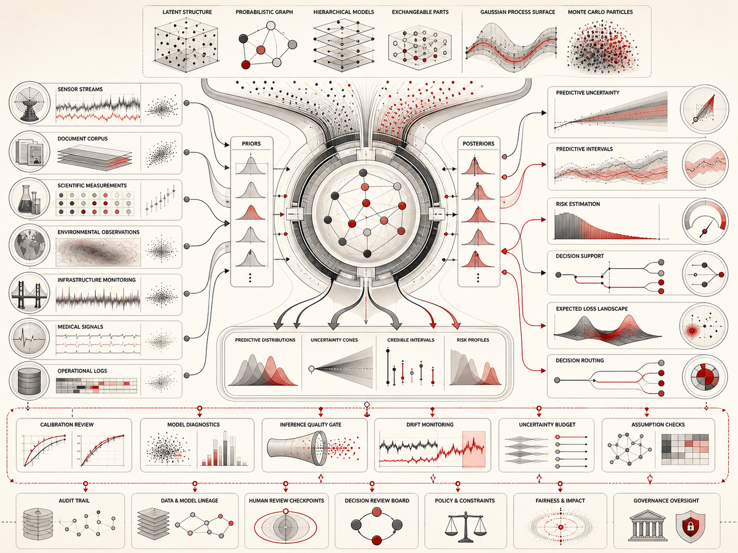
This article develops Probabilistic Machine Learning and Bayesian AI Systems as an advanced article within the Artificial Intelligence Systems knowledge series. It explains probabilistic reasoning, Bayesian inference, priors, likelihoods, posteriors, predictive distributions, latent variables, graphical models, Gaussian processes, Bayesian deep learning, approximate inference, probabilistic programming, calibration, uncertainty communication, expected utility, decision thresholds, monitoring, and institutional accountability. Selected Python and R examples appear here, while the full GitHub repository contains expanded computational scaffolding for Bayesian updating, calibration review, probabilistic forecasting, uncertainty monitoring, decision-support scoring, SQL schemas, documentation templates, and reproducible notebooks.
Why Probabilistic Machine Learning Matters
Probabilistic machine learning matters because most real-world AI systems operate under uncertainty. Data are incomplete. Sensors fail. Labels are noisy. Human judgments vary. Historical records are biased. Systems drift. Future conditions differ from past conditions. Models are misspecified. Rare events matter. Decisions must often be made before perfect information is available.
A deterministic model may produce a single classification, score, ranking, or generated answer. A probabilistic system asks how uncertain that output is, what assumptions generated it, how the uncertainty changes with new evidence, and what action is justified given the stakes. This is especially important when false confidence can cause harm. A medical triage system, climate-risk model, bridge-inspection system, financial fraud detector, ecological monitoring platform, or public-benefits decision-support tool should not merely provide an answer; it should communicate uncertainty, confidence, and evidential limits.
Probabilistic machine learning also supports scientific reasoning. Scientists rarely ask only whether a model predicts correctly. They ask what mechanism could have generated the data, what parameters are plausible, how much uncertainty remains, which hypotheses are supported, and what experiment would reduce uncertainty most. Bayesian AI systems are therefore well suited to fields where evidence accumulates gradually and decisions must be revised as knowledge changes.
In institutional settings, uncertainty is not a technical nuisance to be eliminated from the interface. It is often the most important part of the decision. A public agency deciding where to inspect infrastructure, a hospital deciding whether to escalate a case, a climate adaptation team deciding where to invest, or a financial compliance team deciding which alerts to investigate must know not only what is likely, but how reliable the estimate is and what the cost of being wrong would be.
Prediction \neq Certainty
\]
Interpretation: A model output is not the same as knowledge. Probabilistic AI systems make uncertainty, evidence, assumptions, and decision risk visible.
Probabilistic AI is therefore not just about better mathematics. It is about better judgment under uncertainty. It supports systems that can say: this is likely, this is uncertain, this assumption matters, this evidence is weak, this decision has asymmetric consequences, and this case should be reviewed by a human expert.
Probability as the Language of Uncertainty
Probability gives AI systems a formal language for uncertainty. It allows the system to represent uncertain events, noisy measurements, latent variables, alternative hypotheses, conditional dependencies, and future outcomes. Instead of claiming certainty, the system assigns degrees of belief, frequencies of expected occurrence, or distributions over plausible values.
In probabilistic machine learning, probability may represent several related ideas:
- aleatoric uncertainty: irreducible uncertainty caused by noise, randomness, measurement variation, or inherent variability;
- epistemic uncertainty: reducible uncertainty caused by limited data, weak evidence, model uncertainty, or incomplete knowledge;
- predictive uncertainty: uncertainty about future outputs or outcomes;
- parameter uncertainty: uncertainty about model parameters;
- model uncertainty: uncertainty about which model structure is appropriate;
- decision uncertainty: uncertainty about which action is best under uncertain outcomes and costs.
This distinction is critical for AI governance. Aleatoric uncertainty may need to be communicated and managed. Epistemic uncertainty may require more data, better measurement, additional review, or restricted deployment. A system that cannot distinguish these uncertainties may appear confident where it should defer, escalate, or request more evidence.
| Uncertainty Type | What It Means | Example | Governance Response |
|---|---|---|---|
| Aleatoric uncertainty | Irreducible variability in the process being modeled. | Random variation in weather, measurement noise, or biological response. | Communicate uncertainty and design robust decisions. |
| Epistemic uncertainty | Uncertainty caused by limited knowledge or limited data. | A model is uncertain because few similar cases have been observed. | Collect more data, restrict use, or require expert review. |
| Parameter uncertainty | Uncertainty about model coefficients, weights, rates, or latent quantities. | Uncertain deterioration rate for an infrastructure asset. | Use posterior intervals and sensitivity analysis. |
| Model uncertainty | Uncertainty about which structure or assumptions are appropriate. | Alternative causal structures explain the same data. | Compare models, document assumptions, and avoid false precision. |
| Predictive uncertainty | Uncertainty about a future observation or outcome. | Probability of equipment failure next quarter. | Use prediction intervals and decision thresholds. |
| Decision uncertainty | Uncertainty about which action is justified given risk and cost. | Whether to inspect, monitor, repair, or close an asset. | Use expected loss, human review, and explicit escalation rules. |
Note: Uncertainty is not one thing. Responsible probabilistic AI should distinguish uncertainty caused by noisy reality from uncertainty caused by weak evidence or weak modeling.
Probability also helps prevent overclaiming. A calibrated system can say that an event has a 20 percent probability, not that the event will or will not occur. It can state that an interval contains plausible values, not that a single estimate is final. It can show that two hypotheses remain plausible, not force premature certainty.
Uncertainty = Information\ About\ Limits
\]
Interpretation: Uncertainty is not a weakness to hide. It is information about the limits of current evidence, measurement, model structure, and prediction.
Bayesian Inference and Belief Updating
Bayesian inference treats learning as belief updating. Before observing data, a model has prior beliefs about parameters, hypotheses, or structures. After observing data, those beliefs are updated into a posterior distribution. This posterior becomes the basis for prediction, decision-making, and further learning.
The Bayesian perspective is useful because it makes assumptions visible. Priors encode previous knowledge, domain expertise, physical constraints, institutional history, or modeling assumptions. Likelihoods describe how data would arise under different parameter values or hypotheses. Posteriors combine prior assumptions and observed evidence. Predictions integrate over uncertainty rather than relying on a single best estimate.
This is especially important in low-data settings. When data are limited, prior assumptions matter. A Bayesian system can incorporate domain knowledge rather than pretending that all uncertainty has been resolved by a small dataset. At the same time, priors can introduce bias or inappropriate assumptions if they are poorly chosen. Bayesian inference is powerful because it makes these assumptions explicit, not because it eliminates judgment.
| Bayesian Component | Role | System Example | Governance Question |
|---|---|---|---|
| Prior | Represents assumptions before current evidence. | Engineering knowledge about typical deterioration rates. | Who chose the prior, and is it justified? |
| Likelihood | Connects data to possible parameter values. | Probability of observed sensor readings under different risk states. | Does the likelihood reflect measurement quality and sampling? |
| Posterior | Updated belief after evidence. | Revised probability distribution over asset risk. | How wide is the uncertainty, and what does it imply? |
| Posterior predictive | Prediction that integrates parameter uncertainty. | Forecast probability of future failure or event occurrence. | Is the predictive distribution calibrated? |
| Decision rule | Maps uncertainty to action. | Inspect when expected loss exceeds inspection cost. | Are thresholds and losses explicit and reviewable? |
Note: Bayesian AI is only as responsible as its assumptions, evidence, inference diagnostics, and decision rules.
Bayesian updating also supports sequential learning. A monitoring system can begin with prior knowledge, update as new data arrive, revise predictions, and change actions when uncertainty decreases or risk increases. This is valuable in domains where knowledge accumulates over time: infrastructure inspection, environmental monitoring, public health surveillance, fraud detection, industrial maintenance, and scientific experimentation.
Probabilistic Models and Latent Structure
A probabilistic model describes how data could be generated. It may include observed variables, latent variables, parameters, noise distributions, conditional dependencies, and measurement processes. This generative perspective helps AI systems reason about uncertainty rather than simply fitting input-output mappings.
Latent variables are especially important. A patient’s disease state may be latent while symptoms and tests are observed. Ecological stress may be latent while sensor readings, satellite imagery, and species counts are observed. Infrastructure deterioration may be latent while cracks, vibration, age, material records, and maintenance history are observed. Topic structure may be latent while documents are observed. Probabilistic modeling allows AI systems to infer hidden structure from noisy evidence.
Probabilistic models also support missing-data reasoning. Instead of discarding incomplete records or filling missing values with crude estimates, a probabilistic system can model missingness, uncertainty, and dependencies among variables. This is valuable in institutional systems where complete data are rare and missingness may itself be informative.
| Domain | Observed Evidence | Latent Structure | Why Probabilistic Modeling Helps |
|---|---|---|---|
| Medicine | Symptoms, labs, imaging, clinical notes. | Disease state, severity, treatment response. | Combines noisy evidence and communicates diagnostic uncertainty. |
| Infrastructure | Inspections, sensors, age, traffic, maintenance records. | Deterioration state and failure risk. | Supports inspection prioritization under sparse evidence. |
| Ecology | Species counts, acoustic signals, satellite imagery, field notes. | Habitat condition, biodiversity pressure, ecosystem stress. | Accounts for observation error and incomplete measurement. |
| Finance | Transactions, behavior logs, risk flags, historical outcomes. | Fraud, default risk, hidden exposure. | Estimates uncertain risk and adjusts thresholds by expected loss. |
| Scientific inference | Experiments, simulations, measurements, literature evidence. | Parameters, mechanisms, hypotheses. | Supports hypothesis updating and uncertainty-aware prediction. |
Note: Latent variables are not directly observed. They must be inferred from evidence, assumptions, and model structure.
Probabilistic models also make measurement assumptions explicit. A sensor reading is not reality itself. A label is not always ground truth. A human annotation may contain disagreement. A missing record may reflect administrative failure rather than absence of risk. By modeling the measurement process, probabilistic AI can better distinguish signal from noise.
Probabilistic Graphical Models and Bayesian Networks
Probabilistic graphical models represent relationships among variables using graph structure. Nodes represent variables. Edges represent dependencies. Bayesian networks use directed edges to represent conditional relationships, while Markov networks use undirected edges to represent symmetric dependency structure.
Graphical models are useful because they make assumptions about dependency explicit. A Bayesian network can represent how causes, observations, risks, and outcomes relate. For example, a flood-risk model might include rainfall, soil saturation, drainage capacity, land cover, river level, infrastructure condition, sensor reliability, and observed damage. The graph helps clarify which variables influence which others and how evidence should propagate.
Graphical models also support explainability. A black-box model may output a risk score without showing how evidence interacts. A probabilistic graphical model can expose conditional structure, uncertainty, and evidence pathways. This does not make every model simple, but it creates a more inspectable framework for certain decision-support systems.
| Model Type | Representation | Common Use | Governance Value |
|---|---|---|---|
| Bayesian network | Directed graph of conditional dependencies. | Risk analysis, diagnosis, causal-style reasoning, evidence propagation. | Makes assumptions about dependency explicit. |
| Markov network | Undirected graph of dependency relationships. | Spatial systems, structured prediction, relational dependencies. | Represents interdependence without directional claims. |
| Hidden Markov model | Latent state sequence generating observations. | Speech, sensor monitoring, event sequences, state tracking. | Separates hidden condition from noisy measurement. |
| Dynamic Bayesian network | Bayesian network extended across time. | Monitoring, forecasting, maintenance, public health, environmental systems. | Supports sequential updating and temporal accountability. |
| Factor graph | Variables connected through factor functions. | Probabilistic programming, inference engines, robotics, error correction. | Clarifies how evidence factors combine. |
Note: Graphical models help make uncertainty structure inspectable, but graph choices are assumptions that must be documented and tested.
In governance terms, a graphical model can help reveal where uncertainty enters the system. Is the uncertainty in the measurement? In the causal pathway? In the missing data? In the prior? In the relationship between risk and action? This matters because different uncertainties require different institutional responses.
Graph\ Structure = Assumption\ Structure
\]
Interpretation: A probabilistic graph does not merely visualize variables. It encodes assumptions about dependency, evidence flow, and uncertainty propagation.
Gaussian Processes and Bayesian Nonparametrics
Gaussian processes are probabilistic models over functions. Instead of estimating only a fixed set of parameters, a Gaussian process places a distribution over possible functions that could explain the data. This makes Gaussian processes useful for regression, spatial modeling, uncertainty estimation, Bayesian optimization, active learning, and scientific modeling.
A Gaussian process is especially useful when uncertainty about the function matters. In environmental monitoring, the system may estimate pollution levels between sensor locations. In materials science, it may model expensive experiments. In infrastructure inspection, it may predict deterioration from sparse observations. In optimization, it may decide which experiment to run next by balancing exploration and exploitation.
The advantage is that Gaussian processes provide predictive means and uncertainty estimates. The limitation is computational cost: exact Gaussian process inference can become expensive as dataset size grows. Scalable approximations, sparse methods, kernels, and inducing-point strategies are therefore important in operational systems.
| Use Case | What the Model Estimates | Why Uncertainty Matters | Operational Constraint |
|---|---|---|---|
| Spatial monitoring | Pollution, temperature, moisture, biodiversity, or exposure across space. | Identifies where measurements are sparse or uncertain. | Requires spatial kernels and sensor-quality metadata. |
| Scientific experimentation | Unknown response surface for experiments. | Guides which experiment should be run next. | Must balance exploration, cost, and safety. |
| Infrastructure deterioration | Risk or condition over time and asset characteristics. | Flags assets with high uncertainty as well as high estimated risk. | Needs scalable inference and engineering review. |
| Bayesian optimization | Objective function for expensive evaluation. | Balances known good regions and uncertain promising regions. | Depends on acquisition functions and constraints. |
| Active learning | Where new labels would most reduce uncertainty. | Uses limited labeling budget efficiently. | Needs careful sampling to avoid bias reinforcement. |
Note: Gaussian processes are valuable when uncertainty over functions is operationally important, especially in sparse-data scientific and infrastructure settings.
Bayesian nonparametric methods more broadly allow model complexity to grow with evidence. This can be valuable when the number of clusters, topics, regimes, or latent structures is unknown in advance. But these methods require careful communication: “nonparametric” does not mean assumption-free. It means the model can adapt flexibly under a particular probabilistic structure.
Bayesian Deep Learning and Uncertainty in Neural Systems
Deep learning systems are powerful, but conventional neural networks often provide poorly calibrated confidence. A model may assign high confidence to wrong predictions, out-of-distribution examples, or brittle pattern matches. Bayesian deep learning attempts to bring uncertainty estimation into neural systems by representing uncertainty over weights, functions, predictions, or ensembles.
Bayesian neural networks place distributions over model parameters rather than using a single fixed set of weights. Approximate methods make this more practical, including variational inference, Monte Carlo dropout, deep ensembles, Laplace approximations, stochastic weight averaging, and other uncertainty-aware techniques. These methods vary in mathematical assumptions, computational cost, and reliability.
For AI systems, the key question is not whether a model is “Bayesian” in name. The key question is whether uncertainty estimates are useful, calibrated, monitored, and connected to decisions. A system that estimates uncertainty but ignores it in deployment is not meaningfully uncertainty-aware. Bayesian deep learning should therefore be evaluated as part of a decision workflow.
| Method | Basic Idea | Strength | Limit |
|---|---|---|---|
| Bayesian neural networks | Represent distributions over weights or functions. | Principled uncertainty framing. | Often computationally difficult at scale. |
| Monte Carlo dropout | Use dropout at inference to approximate uncertainty. | Practical and relatively easy to implement. | Approximation quality depends on assumptions. |
| Deep ensembles | Train multiple models and compare predictions. | Often strong empirical uncertainty performance. | Expensive and not fully Bayesian. |
| Laplace approximation | Approximate posterior near an optimum. | Useful for uncertainty around trained parameters. | Local approximation may miss complex posterior structure. |
| Conformal prediction | Produces prediction sets with coverage guarantees under assumptions. | Useful for uncertainty communication and coverage. | Requires careful calibration data and exchangeability assumptions. |
Note: Uncertainty methods should be judged by calibration, coverage, robustness, decision usefulness, and monitoring performance, not by terminology alone.
Bayesian deep learning is especially important for out-of-distribution detection and safety review. A model that is uncertain when it sees unfamiliar conditions can route cases to human review, request more evidence, or abstain. A model that remains confidently wrong under shift may become dangerous in deployment.
Approximate Inference: MCMC, Variational Inference, and Monte Carlo Methods
Bayesian inference often requires integrals that cannot be solved analytically. Approximate inference methods make Bayesian modeling practical. These methods are not merely technical details; they shape the reliability, speed, and credibility of probabilistic AI systems.
Markov chain Monte Carlo methods draw samples from the posterior distribution. These samples can approximate posterior summaries, predictive distributions, and uncertainty intervals. MCMC can be accurate but computationally expensive, and it requires convergence diagnostics.
Variational inference turns inference into optimization. Instead of sampling directly from the true posterior, it chooses an approximate distribution from a family of distributions and optimizes closeness to the target posterior. Variational inference can be faster and more scalable than MCMC, but it may underestimate uncertainty or introduce approximation bias.
Monte Carlo methods approximate expectations through random sampling. They are widely used in Bayesian prediction, uncertainty propagation, simulation, and risk analysis. In AI systems, Monte Carlo methods can help propagate uncertainty from model parameters through predictions and decisions.
| Method | Purpose | Strength | Governance Concern |
|---|---|---|---|
| MCMC | Sample from posterior distributions. | Flexible and often accurate when diagnostics are good. | Requires convergence checks and computational resources. |
| Variational inference | Approximate posterior inference through optimization. | Faster and more scalable for large systems. | May underestimate uncertainty or miss posterior modes. |
| Monte Carlo simulation | Approximate expectations and propagate uncertainty. | Intuitive and broadly applicable. | Requires enough samples and careful interpretation. |
| Laplace approximation | Approximate posterior locally around an optimum. | Computationally efficient in some settings. | Can be misleading for non-Gaussian or multimodal posteriors. |
| Sequential Monte Carlo | Update distributions over time with particles. | Useful for filtering and dynamic systems. | Particle degeneracy and computational cost require monitoring. |
Note: Approximate inference creates a tradeoff among accuracy, speed, scalability, diagnostics, and operational reliability.
Approximate inference is a systems tradeoff. Accuracy, speed, scalability, interpretability, convergence, and operational reliability must be balanced. A method that is mathematically elegant but too slow for deployment may fail operationally. A method that is fast but poorly calibrated may fail institutionally.
Approximation \neq Error\ Free
\]
Interpretation: Approximate Bayesian inference can make uncertainty modeling practical, but approximation error must be diagnosed, documented, and monitored.
Probabilistic Programming Systems
Probabilistic programming systems allow users to specify probabilistic models and perform inference using software frameworks. Instead of manually deriving every inference algorithm, practitioners define the model structure, priors, likelihoods, and observed data. The system then supports sampling, variational inference, diagnostics, posterior prediction, and model checking.
Probabilistic programming is important because it makes Bayesian modeling more reusable and auditable. A model can be expressed as code, versioned, reviewed, tested, and connected to data pipelines. This is especially useful for scientific and institutional applications where assumptions must be documented.
However, probabilistic programming does not remove modeling responsibility. Users must still choose appropriate priors, likelihoods, data transformations, convergence diagnostics, model checks, and decision rules. Poorly specified probabilistic programs can produce misleading certainty, unstable inference, or inappropriate decisions. The software makes Bayesian modeling more accessible; it does not guarantee good Bayesian reasoning.
| System Element | Function | Governance Need | Failure Risk |
|---|---|---|---|
| Model code | Defines priors, likelihoods, and latent structure. | Version control, peer review, documentation. | Hidden assumptions or incorrect model structure. |
| Inference engine | Runs sampling, variational inference, or other methods. | Diagnostics, reproducibility, compute monitoring. | Nonconvergence or approximation error. |
| Posterior checks | Test whether model behavior matches data patterns. | Posterior predictive checks and residual review. | Model appears precise but fits poorly. |
| Decision layer | Maps posterior uncertainty to action. | Threshold documentation and expected-loss review. | Values hidden inside technical parameters. |
| Audit artifacts | Preserve assumptions, outputs, diagnostics, and revisions. | Model cards, system cards, logs, governance reports. | Model cannot be reviewed after deployment. |
Note: Probabilistic programming can improve auditability when model assumptions, inference diagnostics, and decision rules are preserved as reviewable artifacts.
In institutional AI, probabilistic programming can support a different kind of transparency: not a simple explanation of every prediction, but a reproducible record of assumptions, evidence, inference, diagnostics, and decision rules. That record can be reviewed, challenged, revised, and improved.
Bayesian Decision-Making and Expected Utility
Probabilistic prediction becomes operationally meaningful when connected to decisions. A model may estimate that a bridge has a 20 percent probability of serious deterioration, a patient has a 7 percent probability of adverse outcome, or a watershed has a 35 percent probability of flood exceedance. The action depends not only on the probability, but on the cost of false positives, false negatives, intervention, delay, and uncertainty.
Bayesian decision theory connects uncertainty to action through expected utility or expected loss. A high-stakes decision may justify intervention even when probability is moderate. A low-stakes recommendation may tolerate more uncertainty. A public-sector system may require different thresholds because errors are distributed unevenly across communities.
This is where probabilistic AI becomes institutional. The model estimates uncertainty, but the institution defines acceptable risk, legal constraints, ethical obligations, escalation rules, and human review requirements. Bayesian AI systems should not hide value judgments inside thresholds. Decision rules should be explicit, documented, and reviewable.
| Decision Element | Question | Example | Accountability Requirement |
|---|---|---|---|
| Predicted probability | How likely is the outcome? | Probability of failure, illness, fraud, or flooding. | Must be calibrated and communicated clearly. |
| Uncertainty interval | How uncertain is the estimate? | Wide credible interval due to sparse evidence. | Should trigger review when uncertainty is consequential. |
| Loss function | What is the cost of each error? | Missed deterioration costs more than unnecessary inspection. | Costs should be explicit and ethically reviewable. |
| Threshold | When does action occur? | Inspect when expected loss exceeds inspection cost. | Thresholds must be documented and periodically reviewed. |
| Human review | Which cases require expert judgment? | High uncertainty or high impact routes to engineer or clinician. | Review must be meaningful, timely, and empowered. |
Note: Bayesian decision-making makes uncertainty actionable, but action rules encode institutional values and must be governed.
Decision = Probability + Consequence + Responsibility
\]
Interpretation: A probability alone does not determine action. Decision-making also requires consequences, values, legal obligations, and institutional responsibility.
Expected utility is therefore not a neutral substitute for ethics. It is a formal way to expose the tradeoffs that were already present. If a threshold prioritizes efficiency over safety, or cost savings over vulnerable populations, the mathematics does not make that choice neutral. It makes the choice easier to inspect.
Evaluation, Calibration, and Reliability
Probabilistic AI systems must be evaluated differently from deterministic systems. Accuracy alone is insufficient. A model that predicts the correct class but assigns poorly calibrated probabilities can still be dangerous. A system that ranks cases well may still provide unreliable uncertainty intervals. A system that performs well on average may fail under distribution shift or for specific groups.
| Evaluation Dimension | Question | Example Evidence | Governance Relevance |
|---|---|---|---|
| Calibration | Do predicted probabilities match observed frequencies? | Reliability diagrams, expected calibration error, Brier score. | Ensures probabilities can support decisions. |
| Sharpness | Are predictions informative rather than overly broad? | Prediction interval width, entropy, posterior concentration. | Prevents uselessly vague uncertainty estimates. |
| Coverage | Do uncertainty intervals contain true outcomes at expected rates? | Empirical interval coverage. | Tests whether intervals are trustworthy. |
| Discrimination | Can the model separate higher-risk and lower-risk cases? | AUC, precision-recall, ranking metrics. | Supports triage and prioritization. |
| Robustness | Does uncertainty increase under shift or poor evidence? | Out-of-distribution tests, stress tests, perturbation analysis. | Identifies brittle overconfidence. |
| Decision utility | Do probabilistic outputs improve decisions? | Decision curves, expected loss, cost-sensitive evaluation. | Connects model quality to institutional outcomes. |
| Fairness | Are uncertainty and errors uneven across groups? | Subgroup calibration, error gaps, allocation review. | Prevents aggregate calibration from hiding local harm. |
| Governance readiness | Are assumptions, priors, and thresholds documented? | Model cards, prior review, decision-rule logs, audit trails. | Makes uncertainty systems reviewable. |
Note: Probabilistic evaluation should assess whether probabilities, intervals, and uncertainty estimates are reliable enough for the decisions they influence.
Probabilistic evaluation should be connected to the use case. A 90 percent interval that only covers 70 percent of true outcomes is unreliable. A risk score that is calibrated overall but poorly calibrated for a subgroup may be unjust. A model that communicates uncertainty well but is ignored by users may fail in workflow design. Evaluation must therefore include mathematical, operational, and human factors.
Calibration should also be monitored after deployment. A model may be calibrated at launch but become unreliable under drift, changing population structure, sensor degradation, or policy shifts. Probabilistic monitoring should therefore track not only accuracy, but probability reliability over time and across slices.
Calibration\ at\ Launch \neq Calibration\ in\ Production
\]
Interpretation: Probability estimates can decay when data, populations, measurements, or decision processes change. Calibration must be monitored over time.
Governance, Risk, and Institutional Accountability
Probabilistic AI governance requires attention to assumptions. Priors, likelihoods, thresholds, loss functions, evidence sources, uncertainty displays, and escalation rules are all governance objects. They shape system behavior and determine how uncertainty becomes action.
A responsible probabilistic AI system should document:
- model purpose and intended use;
- prior assumptions and their justification;
- likelihood and measurement assumptions;
- data provenance and missing-data handling;
- uncertainty type and interpretation;
- calibration and coverage evidence;
- decision thresholds and loss assumptions;
- subgroup calibration and fairness review;
- human review and escalation rules;
- monitoring for drift and calibration decay;
- rollback and model revision procedures.
Bayesian systems can improve accountability because they expose uncertainty and assumptions. But they can also create a false sense of rigor if complex mathematics hides contested values, poor data, or weak institutional oversight. Governance must therefore treat probabilistic output as decision support, not as unquestionable authority.
| Governance Object | What Must Be Reviewed? | Why It Matters | Audit Artifact |
|---|---|---|---|
| Priors | Assumptions before current evidence. | Can encode domain expertise or bias. | Prior rationale, sensitivity analysis, expert review. |
| Likelihoods | Measurement and data-generation assumptions. | Can misrepresent noise, missingness, or sampling. | Model specification and diagnostic checks. |
| Posteriors | Updated uncertainty after data. | Basis for prediction and decision-making. | Posterior summaries, intervals, diagnostics. |
| Thresholds | Rules connecting probability to action. | Encode risk tolerance and institutional values. | Decision-rule documentation. |
| Calibration | Reliability of probability estimates. | Poor probabilities can mislead decisions. | Reliability diagrams, Brier score, subgroup analysis. |
| Review rules | When humans must intervene. | Protects against over-automation under uncertainty. | Escalation logs and review outcomes. |
Note: Probabilistic governance is assumption governance. The system’s uncertainty estimates are only trustworthy when assumptions, diagnostics, and decisions are reviewable.
NIST’s AI Risk Management Framework remains a prominent voluntary governance reference for mapping, measuring, managing, and governing AI risk across the lifecycle. In 2026 NIST stated that AI RMF 1.0 is being revised and released a concept note for a trustworthy-AI profile focused on critical infrastructure, reinforcing the need for ongoing monitoring, override, incident response, recovery, and change management in deployed systems.
Probabilistic\ Accountability = Assumptions + Evidence + Calibration + Review
\]
Interpretation: Probabilistic AI becomes accountable when its assumptions, evidence base, reliability, and decision pathways are documented and reviewable.
Institutional accountability also requires uncertainty communication. A probability that is technically correct but poorly understood can still mislead. Users may confuse probability with certainty, confidence with truth, uncertainty with ignorance, or risk with destiny. A responsible system should communicate uncertainty in terms that match the user, decision, and consequence.
Common Failure Modes
Probabilistic machine learning often fails when mathematical sophistication is mistaken for institutional reliability. A posterior distribution may look rigorous while resting on weak priors, misspecified likelihoods, biased data, untested calibration, or hidden decision thresholds. Probabilistic output can improve accountability, but only when assumptions and diagnostics remain visible.
| Failure Mode | Description | Likely Consequence | Governance Response |
|---|---|---|---|
| Misleading priors | Priors encode bias, outdated knowledge, or unjustified assumptions. | Posterior results appear evidence-based but are assumption-driven. | Document priors, run sensitivity analysis, involve domain review. |
| Misspecified likelihood | The model misrepresents measurement, sampling, or noise. | Uncertainty estimates become unreliable. | Use posterior predictive checks and measurement review. |
| Approximation error | Inference method distorts posterior uncertainty. | Intervals become too narrow or posterior modes are missed. | Use diagnostics, convergence checks, and alternative inference comparisons. |
| Calibration decay | Probabilities become unreliable after deployment drift. | Decision thresholds become unsafe or unfair. | Monitor calibration over time and across slices. |
| False precision | Complex math creates a sense of certainty not supported by evidence. | Users overtrust estimates and intervals. | Communicate uncertainty limits and evidence quality. |
| Hidden value judgments | Loss functions and thresholds encode ethics or politics invisibly. | Decisions appear neutral but reflect contested priorities. | Make costs, thresholds, and tradeoffs explicit. |
| Ignored uncertainty | System estimates uncertainty but downstream workflow ignores it. | High-uncertainty cases are treated as routine. | Connect uncertainty to review, escalation, or data collection. |
| Aggregate calibration only | Model is calibrated overall but not for subgroups or contexts. | Unequal risk and unfair decisions. | Require subgroup calibration and local reliability review. |
Note: Probabilistic systems can fail by appearing more rigorous than the evidence justifies. Governance must keep assumptions, diagnostics, and decisions visible.
The most important failure mode is not mathematical error alone. It is the transformation of uncertainty into false authority. A probability estimate can be useful, but it can also hide weak data, contested assumptions, or unequal consequences when presented without context.
Limits and Open Problems
Probabilistic machine learning and Bayesian AI systems have important limits. Priors can mislead: poorly chosen priors can encode bias, inappropriate assumptions, or outdated knowledge. Likelihoods can be wrong: a mathematically precise likelihood may still misrepresent measurement, sampling, or causal structure. Approximate inference can distort uncertainty: variational methods, sampling failures, or convergence problems can produce misleading posteriors.
Calibration can decay. Probabilities that were reliable at launch may become unreliable under distribution shift. Uncertainty can be misunderstood: users may confuse probability, confidence, risk, and frequency. Decision thresholds can hide values: expected-loss functions require explicit costs, but those costs may be ethical or political judgments. Complexity can reduce accountability: Bayesian models can become difficult to audit if assumptions, code, and inference diagnostics are poorly documented.
Several open problems remain difficult. How should probabilistic systems communicate uncertainty to non-technical users without oversimplifying? How should institutions govern priors that reflect expert judgment but also social assumptions? How should uncertainty be represented when data are structurally biased rather than merely sparse? How should Bayesian deep learning scale while preserving reliable uncertainty? How should organizations monitor calibration for rare events where outcomes are delayed or hard to observe?
Another open problem is the relationship between probabilistic reasoning and justice. A model may be statistically calibrated but still institutionalize unequal risk burdens. Expected-loss calculations may minimize aggregate loss while imposing disproportionate harms on vulnerable groups. Bayesian AI systems can expose uncertainty, but they cannot by themselves decide what risks are acceptable, who bears them, or who has authority to act.
The goal is not to treat Bayesian AI as inherently superior to all other approaches. The goal is to recognize where uncertainty matters and to design systems that represent, evaluate, communicate, and govern that uncertainty. Probabilistic machine learning gives AI systems a disciplined way to learn from evidence, update beliefs, and support decisions under uncertainty. Responsible deployment requires making the assumptions, uncertainty, thresholds, and consequences visible.
Bayesian Workflow as an AI Lifecycle
Bayesian analysis is often introduced as a formula that converts a prior and likelihood into a posterior. Operationally, it is an iterative workflow. The analyst defines the decision, identifies the data-generating and measurement processes, constructs a generative model, evaluates priors, checks computation, compares simulated and observed data, studies sensitivity, validates predictions, and connects uncertainty to action. Any stage can reveal that the model must be revised.
This workflow perspective matters because a mathematically valid posterior can still be operationally weak. The wrong outcome may be modeled. Measurements may be biased. A likelihood may omit heavy tails or dependence. Priors may encode unrealistic scales. Inference may not converge. A model may reproduce averages while missing rare but consequential behavior. A calibrated probability can still be attached to an unjust decision rule.
| Workflow stage | Primary question | Required evidence |
|---|---|---|
| Problem and decision framing | What decision will the probability influence? | Use case, affected groups, costs, legal duties, escalation rules. |
| Generative and measurement design | How could the observed data have arisen? | Domain model, sampling process, missingness, label and sensor quality. |
| Prior design | What assumptions apply before current evidence? | Domain knowledge, historical evidence, constraints, sensitivity analysis. |
| Inference and computation | Was the intended posterior approximated reliably? | Convergence, effective sample size, divergences, simulation tests. |
| Model criticism | Does the model reproduce relevant features of reality? | Prior and posterior predictive checks, residuals, failure slices. |
| Decision and monitoring | How does uncertainty change action over time? | Loss functions, abstention, review, calibration and drift monitoring. |
The outcome of a Bayesian workflow is therefore not merely a fitted model. It is a reviewable chain connecting assumptions, evidence, computation, prediction, decision, and revision.
Prior Design, Elicitation, and Prior Predictive Checking
Priors can encode scientific knowledge, engineering constraints, historical rates, regularization, physical plausibility, or institutional assumptions. They can also encode bias, outdated practice, or unjustified certainty. A prior should be designed in the scale of the modeled quantity and interpreted through the outcomes it implies.
Prior predictive checking samples parameters from the prior and then simulates data from the likelihood. The resulting outcomes reveal whether the combined assumptions generate impossible failure rates, implausible medical values, unrealistic spatial variation, or excessively narrow predictions before observed data influence the model.
p(y)=\int p(y\mid\theta)p(\theta)\,d\theta
\]
Interpretation: The prior predictive distribution shows what observations the model expects before conditioning on the current dataset.
Weakly informative priors can stabilize estimation without dominating plausible evidence. Strong priors may be justified when mechanisms and measurement are well established, but they require sensitivity analysis. Hierarchical priors can share information across related groups while preserving local variation.
Prior documentation should identify the source, unit, transformation, effective strength, affected populations, and alternatives tested. “Noninformative” is rarely an adequate description because every parameterization and constraint still shapes inference.
Likelihoods, Measurement Error, Missingness, and Selection
The likelihood is a model of how observations arise under different latent states and parameter values. It must represent not only the phenomenon of interest but also the process that measures, labels, samples, and records it. A binary label may contain disagreement. A sensor may drift. A rare event may be underreported. An inspection program may target visibly damaged assets, creating selection bias.
Gaussian noise is convenient but often inappropriate for counts, bounded variables, heavy-tailed errors, zero inflation, censoring, or outliers. Likelihood misspecification can produce narrow intervals and false confidence even when posterior computation is flawless.
Missing data also have mechanisms. Values may be missing independently of the system, related to observed variables, or related to the missing value itself. Administrative absence can indicate low capacity rather than low risk. Treating missingness as random can therefore reproduce institutional blind spots.
A responsible probabilistic system models measurement quality, annotator disagreement, detection probability, censoring, selection, and missingness when these processes materially affect the decision.
Hierarchical Modeling and Partial Pooling
Hierarchical models represent variation across people, sites, assets, hospitals, jurisdictions, devices, or time periods while allowing related groups to share information. Complete pooling assumes groups are identical. No pooling estimates every group independently. Partial pooling learns how much information should be shared.
\theta_j \sim \mathcal{N}(\mu,\tau^2)
\]
Interpretation: Group-specific parameters \(\theta_j\) vary around a population distribution, allowing evidence to be shared without forcing equality.
Partial pooling is valuable when some groups have sparse observations. An asset with little evidence can borrow strength from similar assets while retaining wider uncertainty. A hospital with few cases should not receive an unstable estimate that ignores the broader system.
Pooling choices have fairness implications. Excessive pooling can erase meaningful subgroup differences. No pooling can amplify noise and penalize small groups. Hierarchical structure should reflect causal and institutional relationships rather than being chosen only for predictive convenience.
Hyperpriors, group definitions, exchangeability assumptions, and subgroup diagnostics should be documented because they determine which cases are treated as comparable.
Posterior Predictive Checking and Model Criticism
Posterior predictive checking asks whether data simulated from the fitted model resemble the observed data in features relevant to the intended use. These checks can examine means, tails, extremes, zeros, temporal dependence, subgroup differences, spatial patterns, event clustering, and decision-critical failure modes.
A model can fit aggregate distributions while failing where it matters. An infrastructure model may reproduce average deterioration but miss correlated failures after extreme weather. A clinical model may fit overall event rates while underestimating risk for a subgroup. A fraud model may reproduce common transactions while missing coordinated attacks.
Posterior predictive checks do not prove that a model is true. They expose discrepancies between the model and observations. The analyst must decide which discrepancies require expansion, a different likelihood, new predictors, a revised measurement model, or restricted use.
Model criticism should be continuous. Production data, appeals, human-review outcomes, incidents, and new environments create fresh evidence about where the model fails.
Computational Diagnostics and Simulation-Based Calibration
Bayesian inference is often approximate. Markov chain Monte Carlo, variational inference, Laplace methods, particle methods, and numerical integration can fail in ways that are not visible from posterior summaries alone.
For sampling methods, diagnostics include chain mixing, rank-normalized \(\hat{R}\), effective sample size, autocorrelation, divergences, energy behavior, tree depth, and sensitivity to initialization. A large sample count does not compensate for biased exploration of the posterior.
Simulation-based calibration tests an inference implementation by repeatedly drawing parameters from the prior, simulating data, fitting the model, and checking whether the true simulated parameters occupy the expected ranks within posterior draws. It can expose coding errors and systematic inference bias.
Variational inference requires additional caution because optimization can converge while the approximation underestimates uncertainty or misses posterior modes. Computational diagnostics are part of the evidential chain, not optional engineering metadata.
Model Comparison, Predictive Validation, and Stacking
Bayesian model comparison should focus on predictive adequacy, scientific interpretation, and decision utility rather than declaring one model universally correct. Leave-one-out cross-validation, predictive log density, information criteria, and out-of-sample tests estimate how models generalize under specified conditions.
Bayes factors and marginal likelihoods can be sensitive to prior choices and parameterization. They may be useful in carefully specified hypothesis comparisons, but they should not be treated as assumption-free evidence.
Stacking combines predictions from multiple models using weights selected for predictive performance. Model averaging can represent structural uncertainty when several models remain plausible. These approaches do not eliminate the need to inspect shared failure modes.
Validation should match deployment. Random splits can overstate performance when data are temporal, spatial, grouped, or repeatedly measured. Future-time, new-site, new-device, and subgroup validation may be more relevant than an average held-out score.
Calibration, Sharpness, and Proper Scoring Rules
Calibration asks whether predicted probabilities correspond to observed frequencies. Sharpness asks whether predictions are concentrated enough to be informative. A perfectly broad prediction can achieve coverage while offering little decision value.
Proper scoring rules reward honest probabilistic forecasts. The Brier score evaluates squared error for binary probabilities. Log score strongly penalizes assigning very low probability to events that occur. Continuous ranked probability score evaluates full predictive distributions.
BS=\frac{1}{n}\sum_{i=1}^{n}(p_i-y_i)^2
\]
Interpretation: The Brier score measures the mean squared difference between predicted probabilities and binary outcomes; lower values are better.
Calibration must be evaluated across time, subgroups, sites, severity levels, and evidence quality. Aggregate reliability can hide local overconfidence. Recalibration can improve probabilities, but it should not conceal a model that lacks discrimination or fails under shift.
Conformal Prediction and Coverage Guarantees
Conformal prediction constructs prediction sets or intervals using calibration data and a nonconformity score. Under exchangeability assumptions, it can provide finite-sample marginal coverage without requiring a correct parametric model.
Conformal methods complement rather than replace Bayesian reasoning. Bayesian models represent assumptions, latent structure, and posterior uncertainty. Conformal calibration can wrap a model to provide empirical coverage guarantees under specified conditions. Hybrid systems can use Bayesian uncertainty to adapt interval width while conformal methods calibrate coverage.
Coverage is not universal. Standard guarantees are marginal rather than automatically conditional for every subgroup or context. Distribution shift, time dependence, feedback, and adaptive data collection can violate assumptions. Weighted, adaptive, and group-aware methods require additional evidence.
A conformal interval that covers at the target rate may still be too wide for practical use or fail disproportionately for a vulnerable subgroup. Coverage, width, subgroup behavior, and decision consequences should be reported together.
Selective Prediction, Abstention, and Risk–Coverage
A responsible AI system should sometimes decline to decide. Selective prediction allows a model to issue predictions only for cases meeting a confidence or evidence criterion, routing other cases to additional measurement, human review, or a safer default.
The risk–coverage curve shows the trade-off between the fraction of cases handled automatically and error among those covered. Lower coverage can reduce risk, but only when abstention identifies difficult or unfamiliar cases reliably.
Coverage(\tau)=P(c(x)\geq\tau)
\]
Interpretation: Coverage is the proportion of cases whose confidence or evidence score exceeds the automation threshold \(\tau\).
Abstention is an institutional action, not a blank output. The organization must have reviewers, response times, appeal routes, workload capacity, and authority to override. If uncertain cases are simply delayed or denied service, abstention can transfer risk rather than reduce it.
Risk–coverage performance should be evaluated by subgroup and under distribution shift because some populations may be rejected more often or receive lower-quality review.
Distribution Shift, Out-of-Distribution Risk, and Prior–Data Conflict
Deployment conditions change. Populations, sensors, policies, incentives, climate, disease prevalence, adversarial behavior, and measurement practices can differ from training data. A system can remain numerically confident while its assumptions no longer apply.
Out-of-distribution detection attempts to identify unfamiliar inputs or representations. High predictive entropy, ensemble disagreement, low likelihood, distance measures, and density-ratio methods can provide signals, but none is a universal detector of semantic novelty.
Prior–data conflict occurs when observations are surprising under the prior predictive distribution. It may indicate a poor prior, changed environment, corrupted data, or a genuine rare event. The response should be investigation, not automatic suppression of the evidence.
Shift monitoring should examine input distributions, missingness, residuals, calibration, outcome prevalence, subgroup behavior, reviewer disagreement, and decision consequences. Retraining without causal understanding can reproduce the same failure on newer data.
Causal Bayesian Models, Counterfactuals, and Transportability
Bayesian inference and causal inference are related but distinct. A posterior distribution can quantify uncertainty within a predictive model without establishing that changing an input will change the outcome. Causal claims require assumptions about interventions, confounding, selection, interference, and measurement.
Bayesian causal models can place distributions over treatment effects, latent confounding structures, missing outcomes, and transport parameters. Graphical models can make assumptions inspectable, but a directed edge is not evidence that the causal relation is correct.
Counterfactual decisions often require transportability: whether an effect estimated in one population, time, or institution applies elsewhere. Hierarchical and partial-pooling structures can represent heterogeneity, but external validity still depends on substantive knowledge.
A decision-support system should distinguish prediction, association, causal estimation, and policy simulation. These outputs answer different questions and require different validation.
Sequential Models, State-Space Systems, and Online Updating
Many AI systems observe a changing latent state through noisy measurements. Hidden Markov models, dynamic Bayesian networks, Kalman filters, particle filters, survival models, and state-space models support inference over time.
Sequential updating can improve monitoring, but it can also compound misspecification. A biased sensor or incorrect transition model can repeatedly push the posterior in the wrong direction. Feedback between model decisions and future data can make the observation process endogenous.
Online systems should define update cadence, data-quality gates, forgetting or discounting rules, change-point detection, rollback, and whether a previous posterior is appropriate as the next prior. Structural breaks may require a new model rather than routine updating.
Temporal validation should simulate delays, missing observations, policy changes, and rare events. A sequential model is accountable only when its update history and versioned decisions can be reconstructed.
Value of Information, Active Learning, and Experimental Design
Uncertainty can guide what evidence to collect next. Value-of-information analysis estimates whether the expected improvement in a decision justifies the cost, delay, risk, or burden of additional information.
VOI = \mathbb{E}[L(a_{\mathrm{current}},Y)]-\mathbb{E}[L(a_{\mathrm{new\ evidence}},Y)]-C_{\mathrm{evidence}}
\]
Interpretation: Additional evidence is valuable when expected reduction in decision loss exceeds the cost of acquiring it.
Active learning selects cases whose labels may most improve a model. Bayesian optimization balances exploration and exploitation for expensive experiments. Sensor placement can target locations where predictive uncertainty or decision value is high.
These methods can create sampling bias when only uncertain or high-value cases are observed. They can also concentrate measurement burden on particular communities. Experimental design should therefore include representativeness, consent, safety, and downstream governance.
Robust Bayes, Sensitivity, and Model Ambiguity
Bayesian outputs can be sensitive to priors, likelihoods, link functions, missing-data assumptions, utility values, and model structure. Sensitivity analysis asks whether conclusions change across plausible alternatives.
Robust Bayesian methods can use heavier-tailed likelihoods, contamination models, bounded influence, alternative prior classes, or decision rules that perform acceptably across several models. Model ensembles and scenario ranges can preserve ambiguity instead of collapsing it into one posterior.
Sensitivity should target decisions, not only parameters. A posterior mean may change little while the recommended action changes sharply near a threshold. Conversely, parameter estimates may vary while all plausible models support the same intervention.
When conclusions are fragile, the system should communicate the dependency, seek additional evidence, narrow the use case, or choose a reversible action. False precision is not resolved by adding more decimal places to a posterior summary.
Subgroup Calibration, Fairness, and Distributional Consequences
A system can be calibrated overall while overestimating or underestimating risk for particular groups, sites, devices, or institutions. Small groups may have wide uncertainty and unstable reliability estimates. Historical outcomes may reflect unequal treatment rather than underlying need.
Fairness criteria can conflict. Calibration, equalized error rates, equal allocation, and equal utility may not all be achievable simultaneously when base rates and institutional conditions differ. The appropriate analysis depends on the decision, rights, and consequences.
Bayesian models can represent group uncertainty and share information hierarchically, but priors and pooling choices can reproduce structural assumptions. A model should not treat protected characteristics as interchangeable technical categories without examining the social process that produced the data.
Distributional review should report who receives automated decisions, who is routed to review, who waits longer, who experiences false negatives, and whose outcomes are unavailable for calibration.
Uncertainty Communication and Human Factors
Probabilities, odds, frequencies, intervals, verbal labels, and visualizations are interpreted differently. Users may anchor on a point estimate, ignore interval width, treat a 70 percent probability as certainty, or assume that “low confidence” means low risk.
Communication should match the decision. Natural frequencies can help with diagnostic reasoning. Calibrated probability ranges can support triage. Scenario narratives can explain model ambiguity. Visual intervals should show what quantity is uncertain and whether the range reflects parameters, future outcomes, or model alternatives.
Interface design should avoid decorative uncertainty that does not affect workflow. If a wide interval is displayed but the automation proceeds unchanged, the system is not uncertainty-aware. Reviewers also need training and enough time to interpret the evidence.
Human judgment is itself uncertain and can be overconfident, inconsistent, fatigued, or biased. The objective is a joint human–AI process whose combined decisions are monitored, not an assumption that the human layer automatically corrects the model.
Probabilistic Foundation Models, Generative Systems, and Agents
Foundation models generate probability distributions over tokens or other outputs, but token probability is not automatically calibrated confidence in factual correctness, safety, legal validity, or task completion. Sequence probabilities reflect the model’s training objective and representation, not a complete epistemic assessment.
Sampling temperature, decoding strategy, retrieval, tools, prompts, and system instructions change outputs without necessarily producing a trustworthy probability of correctness. Self-reported confidence can be correlated with performance while remaining vulnerable to prompt framing and distribution shift.
Agentic systems add correlated uncertainty across planning, retrieval, tool selection, execution, and verification. A small error at one stage can alter later observations and decisions. Pipeline-level reliability cannot be inferred by treating component probabilities as independent.
Probabilistic governance for generative systems should combine task-specific evaluation, external verification, calibration where outcomes are measurable, abstention, provenance, tool-result validation, and human authority for consequential actions.
Production Monitoring, Audit Artifacts, and Change Control
A production probabilistic system should preserve the model version, data snapshot, prior specification, likelihood, inference configuration, random seeds, diagnostics, calibration results, decision rule, reviewer action, and final outcome. These artifacts allow a decision to be reconstructed and challenged.
Monitoring should include probability calibration, coverage, interval width, abstention rate, subgroup performance, missingness, input shift, outcome delay, reviewer disagreement, override, incident severity, and unresolved appeals. Metrics should be connected to action thresholds and accountable owners.
Change control matters because recalibration, prior revision, feature changes, sensor replacement, and workflow redesign can alter decisions even when the model name remains the same. Material changes should trigger validation and documentation.
Rollback and decommissioning procedures are necessary when outcomes cannot be observed quickly enough to prove safety. The absence of detected failure is not evidence of reliability when feedback is incomplete.
Mathematical Lens
Bayesian inference begins with Bayes’ theorem.
p(\theta \mid D)
=
\frac{p(D \mid \theta)p(\theta)}{p(D)}
\]
Interpretation: The posterior distribution \(p(\theta \mid D)\) combines the likelihood \(p(D \mid \theta)\), the prior \(p(\theta)\), and the evidence \(p(D)\). The result is an updated belief about parameters \(\theta\) after observing data \(D\).
The evidence normalizes the posterior.
p(D)
=
\int p(D \mid \theta)p(\theta)\,d\theta
\]
Interpretation: The evidence averages the likelihood across all possible parameter values under the prior. It ensures that the posterior is a valid probability distribution.
Bayesian prediction integrates over parameter uncertainty.
p(y_* \mid x_*,D)
=
\int p(y_* \mid x_*,\theta)p(\theta \mid D)\,d\theta
\]
Interpretation: A Bayesian predictive distribution does not rely on one fixed parameter estimate. It averages predictions across plausible parameter values weighted by the posterior.
Bayesian decision-making chooses actions by expected utility or expected loss.
a^*
=
\arg\min_{a \in \mathcal{A}}
\mathbb{E}_{y \sim p(y \mid x,D)}
\left[
L(a,y)
\right]
\]
Interpretation: The best action \(a^*\) minimizes expected loss over uncertain outcomes. This connects probabilistic prediction to responsible decision-making.
Calibration asks whether predicted probabilities match observed frequencies.
P(Y=1 \mid \hat{p}=q)=q
\]
Interpretation: A model is calibrated if, among cases assigned probability \(q\), the event occurs approximately \(q\) of the time. Calibration is essential when probabilities guide decisions.
Bayesian updating can occur sequentially as new evidence arrives.
p(\theta \mid D_{1:t})
\propto
p(D_t \mid \theta)p(\theta \mid D_{1:t-1})
\]
Interpretation: The previous posterior becomes the new prior when fresh data \(D_t\) arrives. This supports continuous monitoring and adaptive AI systems.
Expected calibration error summarizes probability reliability across bins.
ECE
=
\sum_{b=1}^{B}
\frac{|B_b|}{n}
\left|
acc(B_b)-conf(B_b)
\right|
\]
Interpretation: Expected calibration error compares observed accuracy with predicted confidence across probability bins. Lower values indicate better calibration.
Posterior review can be connected to governance thresholds.
Review =
\begin{cases}
1, & \mathbb{E}[\theta \mid D] \geq \tau_R \\
1, & Width(CI_{\theta}) \geq \tau_U \\
1, & ECE \geq \tau_C \\
1, & ExpectedLoss(a) \geq \tau_L \\
0, & \mathrm{otherwise}
\end{cases}
\]
Interpretation: Review can be triggered by high estimated risk, wide uncertainty intervals, poor calibration, or high expected loss.
Variables and System Interpretation
| Symbol or Term | Meaning | Probabilistic Interpretation | System Relevance |
|---|---|---|---|
| \(D\) | Observed data | Measurements, labels, logs, sensor readings, documents, or outcomes. | Evidence used to update beliefs. |
| \(\theta\) | Model parameters | Unknown quantities governing the model. | Object of posterior inference. |
| \(p(\theta)\) | Prior distribution | Belief before observing current data. | Encodes assumptions and domain knowledge. |
| \(p(D \mid \theta)\) | Likelihood | Probability of observing data under parameter values. | Links model assumptions to evidence. |
| \(p(\theta \mid D)\) | Posterior distribution | Updated belief after observing data. | Basis for uncertainty-aware inference. |
| \(p(y_* \mid x_*,D)\) | Posterior predictive distribution | Distribution over future output \(y_*\). | Supports prediction with uncertainty. |
| \(L(a,y)\) | Loss function | Cost of action \(a\) when outcome \(y\) occurs. | Connects uncertainty to decision risk. |
| \(a^*\) | Optimal action | Action minimizing expected loss. | Decision-support recommendation. |
| \(\hat{p}\) | Predicted probability | Model-assigned event probability. | Used for calibration and decision thresholds. |
| \(q\) | Probability level | Confidence bin or predicted probability value. | Used to test calibration. |
| \(CI_{\theta}\) | Credible or uncertainty interval | Range of plausible parameter or risk values under the posterior. | Communicates uncertainty width and review need. |
| \(\tau\) | Threshold | Risk, uncertainty, calibration, or expected-loss boundary. | Turns probabilistic outputs into governance actions. |
Note: Probabilistic variables should be interpreted in relation to evidence quality, uncertainty communication, decision thresholds, and institutional consequences.
Worked Diagnostic: Bayesian Monitoring for Infrastructure Risk
Consider a city using inspection records, structural sensors, traffic, weather, maintenance history, and engineering review to prioritize bridge interventions. Failure events are rare, evidence quality varies, and the cost of a missed deterioration is much greater than the cost of an unnecessary inspection.
Step 1: Define the decision and loss structure
The institution distinguishes routine monitoring, targeted inspection, engineering review, repair planning, load restriction, and emergency closure. False negatives, false positives, delay, disruption, and unequal service consequences are documented.
Step 2: Build the generative and measurement model
Latent deterioration is separated from noisy sensor readings, inconsistent inspections, missing maintenance records, and selective observation of already suspicious assets.
Step 3: Elicit and test priors
Engineering knowledge and historical failure rates inform priors for deterioration, sensor reliability, and group variation. Prior predictive checks reject assumptions that imply impossible rates or implausibly narrow risk.
Step 4: Fit the hierarchical model and diagnose computation
Related bridge classes partially pool information. Chains, effective sample size, divergences, and simulation-based calibration are reviewed before posterior estimates are accepted.
Step 5: Criticize and validate the model
Posterior predictive checks examine extremes, event clustering, weather response, subgroup behavior, and inspection outcomes. Future-time and new-site validation test transportability.
Step 6: Evaluate calibration, coverage, and abstention
Risk probabilities, credible intervals, conformal coverage, and risk–coverage curves are evaluated across asset classes and evidence-quality bands. Wide or unreliable cases route to engineers.
Step 7: Connect posterior uncertainty to action
Expected loss compares inspection, delay, repair, and closure options. Safety and legal constraints override aggregate utility calculations where necessary.
Step 8: Monitor decisions and revise the system
Calibration decay, sensor replacement, overrides, incidents, unresolved cases, and changed climate exposure trigger review, recalibration, model expansion, or suspension.
| Operating mode | Visible benefit | Failure risk |
|---|---|---|
| Point-risk ranking | Simple prioritization. | Hides interval width, evidence quality, subgroup reliability, and asymmetric loss. |
| Probability threshold only | Connects risk to action. | Can automate unfamiliar or poorly calibrated cases and conceal threshold values. |
| Governed Bayesian workflow | Integrates priors, measurement, diagnostics, calibration, expected loss, abstention, review, and change control. | Requires engineering capacity, outcome feedback, audit artifacts, and authority to stop the system. |
The diagnostic demonstrates that posterior risk is one part of a safety system. Evidence quality, computational validity, calibration, consequence, human authority, and institutional capacity determine whether the output can responsibly influence action.
Computational Modeling
Computational modeling can make probabilistic governance concrete. A Bayesian updating workflow can show how prior beliefs change after evidence. A calibration workflow can test whether predicted probabilities match observed outcomes. A decision workflow can connect probabilities to expected loss. A monitoring workflow can flag cases where uncertainty is too high, evidence quality is too low, or calibration has degraded.
The examples below are intentionally lightweight and educational. They do not replace full probabilistic programming systems, hierarchical Bayesian models, Gaussian-process workflows, formal convergence diagnostics, or domain-specific risk models. Their purpose is to show how uncertainty, calibration, and expected loss can be organized as governance signals.
A mature production system would connect these workflows to real data pipelines, model registries, prior-review documents, posterior diagnostics, calibration dashboards, decision logs, human-review records, incident registers, and monitoring systems. The goal is not merely to compute probabilities. The goal is to make uncertainty useful, inspectable, and accountable.
Python Workflow: Bayesian Risk Updating and Calibration Review
The following Python workflow demonstrates Bayesian updating for a simplified binary risk system. It simulates infrastructure assets, updates prior beliefs with observed events, estimates posterior means and credible intervals, evaluates probability calibration across risk bins, and creates expected-loss-based inspection priorities. It is dependency-light so it can be adapted for real monitoring and governance workflows.
from __future__ import annotations

import csv
import math
from collections import defaultdict
from pathlib import Path
from statistics import mean

ARTICLE_ROOT = Path(__file__).resolve().parents[1]
DATA_FILE = ARTICLE_ROOT / "data" / "probabilistic_ai_cases.csv"
TABLES = ARTICLE_ROOT / "outputs" / "tables"

NORMAL_90_Z = 1.6448536269514722

def clamp(value: float, low: float = 0.0, high: float = 1.0) -> float:
    return max(low, min(high, value))

def quantile(values: list[float], probability: float) -> float:
    ordered = sorted(values)
    position = probability * (len(ordered) - 1)
    lower = int(position)
    upper = min(lower + 1, len(ordered) - 1)
    fraction = position - lower
    return ordered[lower] * (1.0 - fraction) + ordered[upper] * fraction

def load_cases(path: Path = DATA_FILE) -> list[dict[str, object]]:
    with path.open(newline="", encoding="utf-8") as handle:
        rows = list(csv.DictReader(handle))

    numeric = [
        "prior_alpha",
        "prior_beta",
        "observations",
        "adverse_events",
        "sensor_risk",
        "evidence_quality",
        "shift_score",
        "calibration_gap",
        "false_negative_cost",
        "inspection_cost",
        "delay_cost",
        "review_capacity",
        "subgroup_reliability",
    ]
    for row in rows:
        for column in numeric:
            row[column] = float(row[column])
        if row["observations"] < row["adverse_events"]:
            raise ValueError("Adverse events cannot exceed observations.")
        if row["prior_alpha"] <= 0 or row["prior_beta"] <= 0:
            raise ValueError("Beta prior parameters must be positive.")
    return rows

def beta_interval(alpha: float, beta: float) -> tuple[float, float, float]:
    """Return Beta posterior mean and a bounded normal-approximation interval."""
    total = alpha + beta
    posterior_mean = alpha / total
    variance = (alpha * beta) / (total * total * (total + 1.0))
    standard_deviation = math.sqrt(max(variance, 0.0))
    lower = clamp(posterior_mean - NORMAL_90_Z * standard_deviation)
    upper = clamp(posterior_mean + NORMAL_90_Z * standard_deviation)
    return posterior_mean, lower, upper

def score_case(row: dict[str, object], case_index: int = 0) -> dict[str, object]:
    observations = int(float(row["observations"]))
    adverse = int(float(row["adverse_events"]))
    alpha_post = float(row["prior_alpha"]) + adverse
    beta_post = float(row["prior_beta"]) + observations - adverse

    posterior_mean, lower, upper = beta_interval(
        alpha_post,
        beta_post,
    )
    interval_width = upper - lower
    evidence_quality = clamp(float(row["evidence_quality"]))
    sensor_risk = clamp(float(row["sensor_risk"]))
    shift_score = clamp(float(row["shift_score"]))
    calibration_gap = clamp(float(row["calibration_gap"]))
    subgroup_reliability = clamp(float(row["subgroup_reliability"]))
    review_capacity = clamp(float(row["review_capacity"]))

    combined_risk = clamp(
        0.64 * posterior_mean
        + 0.21 * sensor_risk
        + 0.15 * shift_score
    )
    uncertainty_burden = clamp(
        0.42 * min(interval_width / 0.50, 1.0)
        + 0.22 * (1.0 - evidence_quality)
        + 0.20 * calibration_gap
        + 0.16 * (1.0 - subgroup_reliability)
    )
    governed_risk = clamp(
        combined_risk * (1.0 + 0.32 * uncertainty_burden)
    )

    expected_miss_loss = (
        governed_risk * float(row["false_negative_cost"])
        + float(row["delay_cost"]) * uncertainty_burden
    )
    expected_inspect_loss = float(row["inspection_cost"])
    decision_margin = expected_miss_loss - expected_inspect_loss

    abstain = (
        interval_width >= 0.30
        or shift_score >= 0.62
        or calibration_gap >= 0.18
        or subgroup_reliability < 0.58
    )
    if governed_risk >= 0.58:
        recommended_action = "engineering_review"
    elif decision_margin > 0:
        recommended_action = "targeted_inspection"
    else:
        recommended_action = "continue_monitoring"

    if abstain:
        recommended_action = "human_review_and_more_evidence"
    if abstain and review_capacity < 0.45:
        recommended_action = "restrict_use_and_escalate_capacity"

    if governed_risk >= 0.62:
        risk_band = "high"
    elif governed_risk >= 0.34:
        risk_band = "moderate"
    else:
        risk_band = "lower"

    return {
        **row,
        "posterior_alpha": round(alpha_post, 4),
        "posterior_beta": round(beta_post, 4),
        "posterior_mean_risk": round(posterior_mean, 4),
        "credible_lower_90": round(lower, 4),
        "credible_upper_90": round(upper, 4),
        "credible_width_90": round(interval_width, 4),
        "combined_risk": round(combined_risk, 4),
        "uncertainty_burden": round(uncertainty_burden, 4),
        "governed_risk": round(governed_risk, 4),
        "expected_miss_loss": round(expected_miss_loss, 2),
        "expected_inspect_loss": round(expected_inspect_loss, 2),
        "decision_margin": round(decision_margin, 2),
        "abstain": int(abstain),
        "recommended_action": recommended_action,
        "risk_band": risk_band,
    }

def calibration_records(scored: list[dict[str, object]]) -> list[dict[str, object]]:
    bins = [
        (0.0, 0.2),
        (0.2, 0.4),
        (0.4, 0.6),
        (0.6, 0.8),
        (0.8, 1.0001),
    ]
    records = []
    for lower, upper in bins:
        subset = [
            row for row in scored
            if lower <= float(row["posterior_mean_risk"]) < upper
        ]
        if subset:
            predicted = mean(float(row["posterior_mean_risk"]) for row in subset)
            observed = mean(
                float(row["adverse_events"]) / max(float(row["observations"]), 1.0)
                for row in subset
            )
            records.append({
                "bin_lower": lower,
                "bin_upper": min(upper, 1.0),
                "cases": len(subset),
                "mean_predicted_probability": round(predicted, 4),
                "mean_observed_rate": round(observed, 4),
                "absolute_calibration_gap": round(abs(predicted - observed), 4),
            })
        else:
            records.append({
                "bin_lower": lower,
                "bin_upper": min(upper, 1.0),
                "cases": 0,
                "mean_predicted_probability": "",
                "mean_observed_rate": "",
                "absolute_calibration_gap": "",
            })
    return records

def group_summary(scored: list[dict[str, object]]) -> list[dict[str, object]]:
    groups: dict[str, list[dict[str, object]]] = defaultdict(list)
    for row in scored:
        groups[str(row["asset_group"])].append(row)

    records = []
    for group, rows in sorted(groups.items()):
        records.append({
            "asset_group": group,
            "cases": len(rows),
            "mean_governed_risk": round(
                mean(float(row["governed_risk"]) for row in rows), 4
            ),
            "mean_credible_width": round(
                mean(float(row["credible_width_90"]) for row in rows), 4
            ),
            "abstention_rate": round(
                mean(float(row["abstain"]) for row in rows), 4
            ),
            "mean_subgroup_reliability": round(
                mean(float(row["subgroup_reliability"]) for row in rows), 4
            ),
        })
    return records

def decision_scenarios(cases: list[dict[str, object]]) -> list[dict[str, object]]:
    scenarios = {
        "Baseline": {
            "evidence_gain": 0.00,
            "shift_reduction": 0.00,
            "calibration_reduction": 0.00,
            "review_gain": 0.00,
        },
        "Additional inspection evidence": {
            "evidence_gain": 0.12,
            "shift_reduction": 0.04,
            "calibration_reduction": 0.03,
            "review_gain": 0.05,
        },
        "Recalibration and shift controls": {
            "evidence_gain": 0.04,
            "shift_reduction": 0.18,
            "calibration_reduction": 0.14,
            "review_gain": 0.06,
        },
        "Expanded human review capacity": {
            "evidence_gain": 0.03,
            "shift_reduction": 0.03,
            "calibration_reduction": 0.04,
            "review_gain": 0.22,
        },
        "Integrated governed workflow": {
            "evidence_gain": 0.15,
            "shift_reduction": 0.18,
            "calibration_reduction": 0.15,
            "review_gain": 0.22,
        },
    }

    records = []
    for scenario_name, settings in scenarios.items():
        for index, base in enumerate(cases):
            row = dict(base)
            row["evidence_quality"] = clamp(
                float(row["evidence_quality"]) + settings["evidence_gain"]
            )
            row["shift_score"] = clamp(
                float(row["shift_score"]) - settings["shift_reduction"]
            )
            row["calibration_gap"] = clamp(
                float(row["calibration_gap"]) - settings["calibration_reduction"]
            )
            row["review_capacity"] = clamp(
                float(row["review_capacity"]) + settings["review_gain"]
            )
            scored = score_case(row, 5000 + index)
            records.append({
                "scenario": scenario_name,
                "case_id": scored["case_id"],
                "posterior_mean_risk": scored["posterior_mean_risk"],
                "credible_width_90": scored["credible_width_90"],
                "uncertainty_burden": scored["uncertainty_burden"],
                "governed_risk": scored["governed_risk"],
                "abstain": scored["abstain"],
                "recommended_action": scored["recommended_action"],
            })
    return records

def write_csv(path: Path, rows: list[dict[str, object]]) -> None:
    path.parent.mkdir(parents=True, exist_ok=True)
    if not rows:
        raise ValueError(f"No rows for {path}")
    with path.open("w", newline="", encoding="utf-8") as handle:
        writer = csv.DictWriter(handle, fieldnames=list(rows[0].keys()))
        writer.writeheader()
        writer.writerows(rows)

def main() -> None:
    cases = load_cases()
    scored = [score_case(row, index) for index, row in enumerate(cases)]
    scored.sort(key=lambda row: float(row["governed_risk"]), reverse=True)

    write_csv(TABLES / "bayesian_asset_diagnostics.csv", scored)
    write_csv(TABLES / "bayesian_calibration_bins.csv", calibration_records(scored))
    write_csv(TABLES / "bayesian_group_summary.csv", group_summary(scored))
    write_csv(TABLES / "bayesian_decision_scenarios.csv", decision_scenarios(cases))

    brier = mean(
        (
            float(row["posterior_mean_risk"])
            - float(row["adverse_events"]) / max(float(row["observations"]), 1.0)
        ) ** 2
        for row in scored
    )
    print("Probabilistic AI workflow complete.")
    print(f"Synthetic Brier score: {brier:.4f}")
    print(TABLES / "bayesian_asset_diagnostics.csv")

if __name__ == "__main__":
    main()
This workflow treats Bayesian risk estimation as a governance problem. It does not rank assets only by point estimates. It also considers uncertainty width, evidence quality, calibration error, expected loss, and review requirements. That mirrors the core argument of the article: probabilistic AI is most valuable when uncertainty changes how institutions act.
R Workflow: Probabilistic Forecast Evaluation
The following R workflow evaluates probabilistic forecasts using Brier score, calibration bins, interval width, predictive entropy, evidence quality, and review flags. It provides a lightweight review structure for probabilistic AI systems that issue risk probabilities or forecasts.
# Base R probabilistic AI calibration and decision cross-check.
args <- commandArgs(trailingOnly = FALSE)
file_arg <- grep("^--file=", args, value = TRUE)

if (length(file_arg) > 0) {
  script_path <- normalizePath(sub("^--file=", "", file_arg[1]), mustWork = TRUE)
  article_root <- normalizePath(file.path(dirname(script_path), ".."), mustWork = TRUE)
} else {
  article_root <- getwd()
}

input_file <- file.path(article_root, "data", "probabilistic_ai_cases.csv")
output_file <- file.path(article_root, "outputs", "tables", "bayesian_diagnostics_r.csv")

cases <- read.csv(input_file, stringsAsFactors = FALSE)

cases$posterior_alpha <- cases$prior_alpha + cases$adverse_events
cases$posterior_beta <- (
  cases$prior_beta + cases$observations - cases$adverse_events
)
cases$posterior_mean_risk <- (
  cases$posterior_alpha /
  (cases$posterior_alpha + cases$posterior_beta)
)
cases$credible_lower_90 <- qbeta(
  0.05,
  cases$posterior_alpha,
  cases$posterior_beta
)
cases$credible_upper_90 <- qbeta(
  0.95,
  cases$posterior_alpha,
  cases$posterior_beta
)
cases$credible_width_90 <- (
  cases$credible_upper_90 - cases$credible_lower_90
)
cases$combined_risk <- pmin(
  1,
  pmax(
    0,
    0.64 * cases$posterior_mean_risk +
    0.21 * cases$sensor_risk +
    0.15 * cases$shift_score
  )
)
cases$uncertainty_burden <- pmin(
  1,
  pmax(
    0,
    0.42 * pmin(cases$credible_width_90 / 0.50, 1) +
    0.22 * (1 - cases$evidence_quality) +
    0.20 * cases$calibration_gap +
    0.16 * (1 - cases$subgroup_reliability)
  )
)
cases$governed_risk <- pmin(
  1,
  cases$combined_risk * (1 + 0.32 * cases$uncertainty_burden)
)
cases$abstain <- as.integer(
  cases$credible_width_90 >= 0.30 |
  cases$shift_score >= 0.62 |
  cases$calibration_gap >= 0.18 |
  cases$subgroup_reliability < 0.58
)

dir.create(dirname(output_file), recursive = TRUE, showWarnings = FALSE)
write.csv(cases, output_file, row.names = FALSE)

cat("Base R probabilistic AI diagnostics complete.\n")
cat(output_file, "\n")
This R workflow mirrors the probabilistic-governance structure in a compact form. It summarizes forecast reliability by calibration bin and risk group so probability quality, observed outcomes, Brier score, entropy, interval width, empirical coverage, evidence quality, and review status can be interpreted together.
Go Workflow: Lightweight Bayesian Decision and Calibration Service
The Go workflow provides a dependency-free scoring service for posterior risk, interval-width review, expected-loss comparison, evidence-quality checks, and abstention. It is intended as a transparent systems example rather than a substitute for a full probabilistic-programming engine.
package main

import (
	"encoding/csv"
	"fmt"
	"math"
	"os"
	"path/filepath"
	"strconv"
)

func parse(record map[string]string, key string) float64 {
	value, err := strconv.ParseFloat(record[key], 64)
	if err != nil {
		panic(fmt.Errorf("%s: %w", key, err))
	}
	return value
}

func clamp(value float64) float64 {
	return math.Max(0, math.Min(1, value))
}

func main() {
	input := filepath.Join("..", "data", "probabilistic_ai_cases.csv")
	output := filepath.Join("..", "outputs", "tables", "bayesian_scores_go.csv")

	file, err := os.Open(input)
	if err != nil {
		panic(err)
	}
	defer file.Close()

	reader := csv.NewReader(file)
	rows, err := reader.ReadAll()
	if err != nil {
		panic(err)
	}
	headers := rows[0]

	out, err := os.Create(output)
	if err != nil {
		panic(err)
	}
	defer out.Close()

	writer := csv.NewWriter(out)
	defer writer.Flush()
	writer.Write([]string{
		"case_id",
		"posterior_mean_risk",
		"combined_risk",
		"uncertainty_burden",
		"governed_risk",
		"abstain",
		"recommended_action",
	})

	for _, row := range rows[1:] {
		record := map[string]string{}
		for index, header := range headers {
			record[header] = row[index]
		}

		alpha := parse(record, "prior_alpha") + parse(record, "adverse_events")
		beta := parse(record, "prior_beta") +
			parse(record, "observations") -
			parse(record, "adverse_events")
		posteriorMean := alpha / (alpha + beta)
		evidence := clamp(parse(record, "evidence_quality"))
		shift := clamp(parse(record, "shift_score"))
		calibrationGap := clamp(parse(record, "calibration_gap"))
		subgroupReliability := clamp(parse(record, "subgroup_reliability"))
		sensorRisk := clamp(parse(record, "sensor_risk"))

		combinedRisk := clamp(
			0.64*posteriorMean +
				0.21*sensorRisk +
				0.15*shift,
		)
		approximateWidth := 3.29 * math.Sqrt(
			(alpha*beta)/
				(math.Pow(alpha+beta, 2)*(alpha+beta+1)),
		)
		uncertaintyBurden := clamp(
			0.42*clamp(approximateWidth/0.50) +
				0.22*(1-evidence) +
				0.20*calibrationGap +
				0.16*(1-subgroupReliability),
		)
		governedRisk := clamp(
			combinedRisk * (1 + 0.32*uncertaintyBurden),
		)

		abstain := approximateWidth >= 0.30 ||
			shift >= 0.62 ||
			calibrationGap >= 0.18 ||
			subgroupReliability < 0.58

		expectedMissLoss := governedRisk*parse(record, "false_negative_cost") +
			parse(record, "delay_cost")*uncertaintyBurden
		action := "continue_monitoring"
		if expectedMissLoss > parse(record, "inspection_cost") {
			action = "targeted_inspection"
		}
		if governedRisk >= 0.58 {
			action = "engineering_review"
		}
		if abstain {
			action = "human_review_and_more_evidence"
		}

		writer.Write([]string{
			record["case_id"],
			fmt.Sprintf("%.4f", posteriorMean),
			fmt.Sprintf("%.4f", combinedRisk),
			fmt.Sprintf("%.4f", uncertaintyBurden),
			fmt.Sprintf("%.4f", governedRisk),
			strconv.FormatBool(abstain),
			action,
		})
	}

	fmt.Println("Go probabilistic AI scoring complete.")
	fmt.Println(output)
}
GitHub Repository
The article body includes selected computational examples so the conceptual and mathematical argument remains readable. The full repository can hold expanded workflows for Bayesian updating, calibration review, probabilistic forecasting, uncertainty monitoring, Bayesian networks, Gaussian-process examples, approximate inference diagnostics, probabilistic programming metadata, decision-support governance, and reproducible uncertainty reports.
Complete Code RepositoryThe full code distribution for this article includes Python, R, SQL, Rust, Go, Julia, TypeScript, C++, documentation templates, and advanced notebooks for studying probabilistic machine learning, Bayesian inference, uncertainty quantification, calibration, probabilistic forecasting, decision thresholds, expected loss, model diagnostics, and accountable Bayesian AI governance.
From Certainty to Accountable Uncertainty
Probabilistic machine learning and Bayesian AI systems show why trustworthy artificial intelligence cannot be built only around point predictions, classifications, rankings, or generated answers. Many important systems operate where evidence is partial, outcomes are delayed, measurements are noisy, and decisions carry asymmetric consequences. In those settings, uncertainty is not a secondary feature. It is part of the decision itself.
The central lesson is that uncertainty must be represented, evaluated, communicated, and governed. Bayesian inference gives AI systems a disciplined way to update beliefs as evidence changes. Probabilistic forecasting gives systems a way to express future risk. Calibration tells whether probabilities can be trusted. Expected loss connects uncertainty to action. Human review protects cases where uncertainty, consequence, or evidence quality exceeds the system’s authority.
This article also shows why probabilistic AI is not automatically responsible. A Bayesian model can still encode biased priors, misspecified likelihoods, poor measurements, weak diagnostics, hidden value judgments, and misleading thresholds. Mathematical rigor must be matched by institutional rigor. Assumptions should be documented. Calibration should be monitored. Thresholds should be justified. Uncertainty should trigger review when consequences matter.
The strongest probabilistic AI systems will not be those that merely produce more sophisticated probability scores. They will be those that use uncertainty to improve accountability: making evidence limits visible, preventing false confidence, identifying where more information is needed, and connecting probabilistic reasoning to responsible action.
Within the Artificial Intelligence Systems knowledge series, this article belongs near Machine Learning Foundations: How Systems Learn from Data, Model Training, Optimization, and Evaluation, Model Validation, Benchmarking, and Generalization Theory, Calibration, Uncertainty, and Probability in AI Systems, Artificial Intelligence in Decision Support Systems, Data Governance, Provenance, and Lineage in AI Systems, Model Monitoring, Drift, and AI Observability, and AI Governance and Regulatory Systems. It provides the uncertainty-reasoning layer for understanding how AI systems learn from evidence, quantify risk, and support decisions without pretending certainty.
A Practical Method for Building a Governed Probabilistic AI System
1. Define the decision, affected parties, and unacceptable outcomes
Specify what action the model may influence, who bears errors, legal and ethical constraints, and which decisions remain human.
2. Define the target, data-generating process, and measurement process
Separate the latent phenomenon from labels, sensors, administrative records, selection, missingness, and feedback.
3. Construct the generative model
Document variables, dependence, time, groups, causal claims, observation noise, and alternative structures.
4. Elicit, justify, and stress-test priors
Use domain knowledge and prior predictive checks; record source, effective strength, alternatives, and affected groups.
5. Fit the model and verify computation
Review convergence, effective sample size, divergences, approximation quality, initialization, and simulation-based calibration.
6. Criticize the model with predictive checks
Compare simulated and observed data for averages, tails, rare events, dependence, subgroups, and decision-critical failures.
7. Validate under deployment-like conditions
Use future-time, new-site, new-device, subgroup, stress, and shift tests rather than relying only on random holdouts.
8. Evaluate probability quality
Assess calibration, proper scoring rules, sharpness, coverage, interval width, discrimination, and subgroup reliability.
9. Define abstention, escalation, and evidence collection
Route unfamiliar, high-uncertainty, high-impact, or poorly supported cases to meaningful review or additional measurement.
10. Connect probabilities to transparent decision rules
Document expected loss, thresholds, safety constraints, distributional consequences, and override authority.
11. Preserve audit artifacts and monitor production behavior
Version priors, data, code, diagnostics, calibration, decisions, reviews, incidents, appeals, and changes.
12. Reassess, revise, restrict, or decommission
Use outcome feedback and governance review to update the system; suspend it when evidence is insufficient or harm cannot be controlled.
Common Pitfalls in Probabilistic AI Deployment
- Treating a posterior as proof: The posterior is conditional on priors, likelihood, data, computation, and model structure.
- Skipping prior predictive checks: Priors can imply impossible outcomes even when parameter values appear numerically modest.
- Modeling the outcome but not its measurement: Sensor error, label disagreement, selection, and missingness can dominate uncertainty.
- Reporting intervals without checking coverage: An interval is not trustworthy merely because software produced it.
- Using one calibration score: Aggregate ECE can hide time, site, subgroup, severity, and evidence-quality failures.
- Confusing Bayesian uncertainty with conformal coverage: They answer different questions and rely on different assumptions.
- Automating every case: A system without abstention can remain confidently wrong under novelty or weak evidence.
- Ignoring computational diagnostics: Nonconvergence and approximation error can make posterior summaries meaningless.
- Using random validation for structured deployment: Temporal, spatial, grouped, and institutional shifts require matched validation.
- Hiding values inside loss functions: Thresholds and utilities allocate risk and must be publicly reviewable where decisions are consequential.
- Assuming human review is automatically safe: Reviewers need capacity, authority, training, feedback, and monitored outcomes.
- Monitoring inputs but not decisions: Calibration, abstention, overrides, appeals, incidents, and downstream harm must remain visible.
The central mistake is to treat uncertainty quantification as a decorative output rather than a governed chain connecting evidence, assumptions, computation, prediction, decision, and accountability.
Related Articles
- Artificial Intelligence Systems
- Machine Learning Foundations: How Systems Learn from Data
- Model Training, Optimization, and Evaluation
- Model Validation, Benchmarking, and Generalization Theory
- Calibration, Uncertainty, and Probability in AI Systems
- Representation Learning and Embedding Spaces
- AI Safety and System Reliability
- Explainable AI and Model Interpretability
- Artificial Intelligence in Decision Support Systems
- Data Governance, Provenance, and Lineage in AI Systems
Further Reading
- Geifman, Y. and El-Yaniv, R. (2019) SelectiveNet: A Deep Neural Network with an Integrated Reject Option. Available at: https://proceedings.mlr.press/v97/geifman19a.html
- Lakshminarayanan, B., Pritzel, A. and Blundell, C. (2017) Simple and Scalable Predictive Uncertainty Estimation Using Deep Ensembles. Available at: https://proceedings.neurips.cc/paper/2017/hash/9ef2ed4b7fd2c810847ffa5fa85bce38-Abstract.html
- Talts, S. et al. (2018) Validating Bayesian Inference Algorithms with Simulation-Based Calibration. Available at: https://arxiv.org/abs/1804.06788
- Angelopoulos, A.N. and Bates, S. (2021) A Gentle Introduction to Conformal Prediction and Distribution-Free Uncertainty Quantification. Available at: https://arxiv.org/abs/2107.07511
- National Institute of Standards and Technology (2026) AI Risk Management Framework. Available at: https://www.nist.gov/itl/ai-risk-management-framework
- PyMC Developers (2026) Prior and Posterior Predictive Checks. Available at: https://www.pymc.io/projects/docs/en/stable/learn/core_notebooks/posterior_predictive.html
- Stan Development Team (2026) Simulation-Based Calibration Checking. Available at: https://mc-stan.org/docs/stan-users-guide/simulation-based-calibration.html
- Stan Development Team (2026) Posterior and Prior Predictive Checks. Available at: https://mc-stan.org/docs/stan-users-guide/posterior-predictive-checks.html
- Gelman, A. et al. (2026) Bayesian Workflow. Available at: https://research.aalto.fi/en/publications/bayesian-workflow/
- Murphy, K.P. (2022) Probabilistic Machine Learning: An Introduction. MIT Press. Available at: https://probml.github.io/pml-book/book1.html
- Bishop, C.M. (2006) Pattern Recognition and Machine Learning. Springer. Available at: https://www.microsoft.com/en-us/research/wp-content/uploads/2006/01/Bishop-Pattern-Recognition-and-Machine-Learning-2006.pdf
- Pearl, J. (1988) Probabilistic Reasoning in Intelligent Systems: Networks of Plausible Inference. Morgan Kaufmann. Available at: https://www.sciencedirect.com/book/monograph/9780080514895/probabilistic-reasoning-in-intelligent-systems
- Rasmussen, C.E. and Williams, C.K.I. (2006) Gaussian Processes for Machine Learning. MIT Press. Available at: https://gaussianprocess.org/gpml/
- Blei, D.M., Kucukelbir, A. and McAuliffe, J.D. (2017) ‘Variational Inference: A Review for Statisticians’, Journal of the American Statistical Association. Available at: https://arxiv.org/abs/1601.00670
- Gal, Y. and Ghahramani, Z. (2016) ‘Dropout as a Bayesian Approximation: Representing Model Uncertainty in Deep Learning’, Proceedings of the 33rd International Conference on Machine Learning. Available at: https://proceedings.mlr.press/v48/gal16.html
- Carpenter, B. et al. (2017) ‘Stan: A Probabilistic Programming Language’, Journal of Statistical Software. Available at: https://www.jstatsoft.org/article/view/v076i01
- NIST (2023) Artificial Intelligence Risk Management Framework (AI RMF 1.0). Available at: https://www.nist.gov/publications/artificial-intelligence-risk-management-framework-ai-rmf-10
References
- Geifman, Y. and El-Yaniv, R. (2019) SelectiveNet: A Deep Neural Network with an Integrated Reject Option. Available at: https://proceedings.mlr.press/v97/geifman19a.html
- Lakshminarayanan, B., Pritzel, A. and Blundell, C. (2017) Simple and Scalable Predictive Uncertainty Estimation Using Deep Ensembles. Available at: https://proceedings.neurips.cc/paper/2017/hash/9ef2ed4b7fd2c810847ffa5fa85bce38-Abstract.html
- Talts, S. et al. (2018) Validating Bayesian Inference Algorithms with Simulation-Based Calibration. Available at: https://arxiv.org/abs/1804.06788
- Angelopoulos, A.N. and Bates, S. (2021) A Gentle Introduction to Conformal Prediction and Distribution-Free Uncertainty Quantification. Available at: https://arxiv.org/abs/2107.07511
- National Institute of Standards and Technology (2026) AI Risk Management Framework. Available at: https://www.nist.gov/itl/ai-risk-management-framework
- PyMC Developers (2026) Prior and Posterior Predictive Checks. Available at: https://www.pymc.io/projects/docs/en/stable/learn/core_notebooks/posterior_predictive.html
- Stan Development Team (2026) Simulation-Based Calibration Checking. Available at: https://mc-stan.org/docs/stan-users-guide/simulation-based-calibration.html
- Stan Development Team (2026) Posterior and Prior Predictive Checks. Available at: https://mc-stan.org/docs/stan-users-guide/posterior-predictive-checks.html
- Gelman, A. et al. (2026) Bayesian Workflow. Available at: https://research.aalto.fi/en/publications/bayesian-workflow/
- Bishop, C.M. (2006) Pattern Recognition and Machine Learning. Springer. Available at: https://www.microsoft.com/en-us/research/wp-content/uploads/2006/01/Bishop-Pattern-Recognition-and-Machine-Learning-2006.pdf
- Blei, D.M., Kucukelbir, A. and McAuliffe, J.D. (2017) ‘Variational Inference: A Review for Statisticians’, Journal of the American Statistical Association. Available at: https://arxiv.org/abs/1601.00670
- Carpenter, B. et al. (2017) ‘Stan: A Probabilistic Programming Language’, Journal of Statistical Software. Available at: https://www.jstatsoft.org/article/view/v076i01
- Gal, Y. and Ghahramani, Z. (2016) ‘Dropout as a Bayesian Approximation: Representing Model Uncertainty in Deep Learning’, Proceedings of the 33rd International Conference on Machine Learning. Available at: https://proceedings.mlr.press/v48/gal16.html
- Gelman, A. et al. (2015) ‘Stan: A Probabilistic Programming Language for Bayesian Inference and Optimization’. Available at: https://sites.stat.columbia.edu/gelman/research/published/stan_jebs_2.pdf
- Murphy, K.P. (2022) Probabilistic Machine Learning: An Introduction. MIT Press. Available at: https://probml.github.io/pml-book/book1.html
- Pearl, J. (1988) Probabilistic Reasoning in Intelligent Systems: Networks of Plausible Inference. Morgan Kaufmann. Available at: https://www.sciencedirect.com/book/monograph/9780080514895/probabilistic-reasoning-in-intelligent-systems
- PyMC Developers (2026) PyMC: Bayesian Modeling and Probabilistic Programming in Python. Available at: https://www.pymc.io/
- Rasmussen, C.E. and Williams, C.K.I. (2006) Gaussian Processes for Machine Learning. MIT Press. Available at: https://gaussianprocess.org/gpml/
- Stan Development Team (2026) Stan: Software for Bayesian Data Analysis. Available at: https://mc-stan.org/