Sensitivity Analysis in Systems Models: Understanding Model Robustness - Sustainable Catalyst

Last Updated April 22, 2026

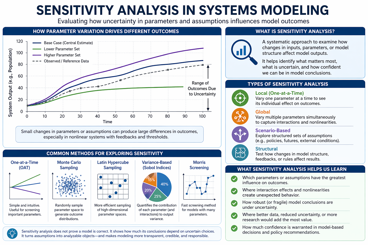
Sensitivity analysis is a methodological technique used to evaluate how changes in model parameters, assumptions, or structural choices influence simulation outcomes. Because systems models depend on estimated variables, theoretical assumptions, and often incomplete data, their results are necessarily conditional rather than absolute. Sensitivity analysis provides a systematic way to examine how strongly those conditions shape model behavior, thereby revealing which assumptions matter most, which conclusions remain robust, and which results are highly contingent on uncertain inputs.

In complex systems modeling, uncertainty is not a peripheral issue but a defining condition of analysis. Environmental variability, behavioral adaptation, technological change, institutional response, and policy intervention all introduce uncertainty into model construction and interpretation. Sensitivity analysis therefore plays a critical role in determining whether model conclusions reflect durable structural relationships or merely the particular parameter values chosen by the analyst.

Methodological research on sensitivity analysis has developed across engineering, climate science, economics, risk analysis, and computational modeling. Institutions such as the MIT System Dynamics Group, the Santa Fe Institute, and the Intergovernmental Panel on Climate Change (IPCC) routinely rely on sensitivity analysis to evaluate the robustness of conclusions drawn from complex systems models.

Within the broader Systems Modeling knowledge series, sensitivity analysis serves as one of the central research practices for testing how models behave under uncertainty and for determining whether their insights are analytically credible.

Text-free dashboard-style illustration with a large multi-line trend chart and uncertainty bands, colored sidebar icons, small sampling and chart tiles, and checklist-style status marks. — Abstract visual representation of sensitivity analysis in systems modeling, showing parameter variation, uncertainty bands, sampling methods, comparative outcomes, and robustness checks without text labels.

This article is part of the Systems Modeling knowledge series.

The Role of Uncertainty in Systems Modeling

All models simplify reality. Parameters such as growth rates, behavioral responses, learning effects, resource availability, discount rates, infrastructure reliability, or technological change must be estimated from incomplete evidence, inferred from theory, or chosen from plausible ranges rather than known with certainty. As a result, model outcomes may vary substantially depending on the values assigned to these assumptions.

Sensitivity analysis addresses this problem by examining how simulation results change when those values are varied systematically. Rather than relying on a single parameterization, analysts explore ranges of plausible values in order to determine whether model conclusions remain stable across uncertainty.

This distinction is fundamental. A model may appear precise while still being highly fragile. Sensitivity analysis helps reveal whether the model’s conclusions are structurally meaningful or simply artifacts of particular assumptions. In this respect, it extends the logic developed in Why Complex Systems Require Modeling and Scenario Modeling and Simulation by shifting attention from model outputs alone to the stability of those outputs under uncertainty.

Types of Sensitivity Analysis

Several major approaches are used to evaluate model sensitivity, each suited to different analytical purposes.

Local sensitivity analysis examines how small changes in a single parameter affect model outcomes while other parameters are held constant. This approach is useful for identifying nearby gradients of influence and for diagnosing which variables have strong marginal effects.

Global sensitivity analysis evaluates how simultaneous variation across multiple parameters influences outcomes. Because complex systems often exhibit interaction effects, nonlinearities, and threshold behavior, global methods are especially important when the influence of one parameter depends on the values of others.

Scenario-based sensitivity analysis explores model behavior across structured sets of assumptions representing alternative futures, policy regimes, or environmental conditions. This approach often overlaps with scenario analysis but focuses more explicitly on how sensitive results are to those structured assumption sets.

Structural sensitivity analysis examines how changes in model form, causal relationships, or representational choices alter conclusions. This is particularly important when model structure itself is uncertain rather than merely the value of individual parameters.

Each of these approaches offers a different perspective on model fragility, robustness, and interpretive confidence.

Identifying Key Drivers of System Behavior

One of the principal aims of sensitivity analysis is to identify which assumptions or variables most strongly influence model behavior. In many complex systems, a relatively small number of parameters may account for much of the variation in outcomes.

For example, in climate models, assumptions about emissions pathways, climate sensitivity, energy transition speed, and land-use change may dominate long-term projections. In economic models, productivity growth, investment behavior, expectations, and institutional response may strongly shape trajectories. In infrastructure and operational systems, utilization rates, failure probabilities, and service times may determine performance.

By identifying these high-leverage assumptions, sensitivity analysis helps researchers focus attention on the drivers that matter most. It also allows policymakers to distinguish between conclusions that are broadly robust and those that rest on parameters that remain poorly understood.

This analytical function connects closely to the broader concern with core principles of systems modeling, especially leverage, feedback, and nonlinearity.

Techniques and Computational Methods

Modern sensitivity analysis often depends on computational experimentation. Analysts run repeated simulations while varying one or more parameters across specified ranges, thereby generating an ensemble of outcomes rather than a single deterministic trajectory.

Common methods include:

one-at-a-time parameter variation
Monte Carlo simulation
Latin hypercube sampling
variance-based global sensitivity methods
screening techniques for high-dimensional models such as Morris-style elementary effects

These approaches allow analysts to explore large parameter spaces and to estimate how much of the variation in model outcomes is attributable to particular assumptions or combinations of assumptions. In effect, the model becomes an experimental environment in which uncertainty can be studied systematically.

This is especially important in complex systems, where interactions among parameters often produce nonlinear responses that cannot be inferred from intuition alone.

Interpretation and Model Robustness

Sensitivity analysis plays a central role in assessing whether model results are robust.

If major conclusions remain stable across a wide range of plausible assumptions, analysts can have greater confidence that the model is capturing structural features of the system rather than merely reflecting arbitrary inputs. If, however, small changes in assumptions produce large differences in outcome, those conclusions must be treated with caution.

This distinction is crucial for responsible model interpretation. Sensitivity analysis helps separate structural insight from parametric fragility. It also prevents false confidence by showing that apparent precision in a model output may conceal deep instability underneath.

For this reason, sensitivity analysis should not be treated as a technical add-on. It is one of the core disciplines through which complex systems modeling earns epistemic credibility.

Relationship to Calibration, Validation, and Uncertainty

Sensitivity analysis is closely related to, but distinct from, several other methodological practices.

Calibration concerns the adjustment of parameter values so that model behavior aligns with empirical observations or known system patterns. Validation concerns whether the model represents the system adequately for the intended purpose. Uncertainty analysis examines the range and character of uncertainty embedded in inputs, structure, and interpretation.

Sensitivity analysis intersects with all three, but its central question is different: How much do conclusions change when assumptions are changed?

This makes it a bridge between model construction and model interpretation. It reveals whether calibrated parameters exert disproportionate influence, whether validated model behavior remains stable under perturbation, and whether uncertainty meaningfully alters the conclusions drawn from the model.

For that reason, this article sits naturally between Scenario Modeling and Simulation and later discussions of Calibration and Validation of Models and Uncertainty and Model Interpretation.

Educational infographic about sensitivity analysis in systems modeling, showing outcome divergence under parameter variation, types of sensitivity analysis, common methods such as Monte Carlo and Latin hypercube sampling, and what sensitivity analysis helps reveal. — Infographic showing how sensitivity analysis tests the robustness of systems-model results by varying parameters, assumptions, and model structures.

Applications in Policy and Sustainability Research

Sensitivity analysis is especially important in policy modeling because policy recommendations often depend on uncertain assumptions about systems that are themselves changing.

Climate policy, energy transitions, infrastructure planning, biodiversity management, macroeconomic forecasting, and public health preparedness all rely on models whose outputs can shape real-world decisions. In such contexts, it is not enough to ask what the model predicts. One must also ask how strongly that prediction depends on uncertain assumptions.

By explicitly examining uncertainty, sensitivity analysis helps policymakers understand which findings are robust, which depend on controversial premises, and which should be treated as provisional. This transparency strengthens the credibility of model-based reasoning and supports more responsible decision-making under uncertainty.

Within the Sustainable Catalyst framework, sensitivity analysis is therefore indispensable for connecting formal modeling to ethical and defensible long-term strategy.

Global Sensitivity and Complex Systems

Sensitivity analysis becomes especially important in complex systems because parameter effects are often interactive rather than isolated.

In linear models, one parameter may have a relatively predictable effect. In nonlinear systems, however, the influence of one variable may depend on the values of many others. Feedback loops, thresholds, adaptive response, and path dependence can create interaction effects that local analysis alone will miss.

This is why global sensitivity methods are often more appropriate for complex systems research. They help reveal not only which assumptions matter, but how assumptions combine to shape trajectories, tipping points, or emergent patterns.

This point is especially relevant for models discussed elsewhere in the series, including system dynamics modeling, agent-based modeling, network models, discrete event simulation, and hybrid modeling approaches.

Methodological Limits and Responsible Use

Although sensitivity analysis strengthens model interpretation, it does not solve every methodological problem.

A model may be insensitive and still wrong if its structure is fundamentally misspecified. Likewise, a model may show sensitivity because it is honestly representing deep uncertainty rather than because it is poorly built. Sensitivity results therefore require interpretation rather than automatic judgment.

Analysts must also choose parameter ranges carefully. If ranges are implausibly narrow, the analysis may create false confidence. If they are implausibly broad, the results may become difficult to interpret. Responsible sensitivity analysis requires clear theoretical justification, careful documentation, and transparency about why particular assumptions were varied.

In this sense, sensitivity analysis is best understood as a discipline of interpretive rigor rather than a mere computational routine.

Implications for Research Practice

Sensitivity analysis improves research practice by making assumptions visible, contestable, and analyzable. It encourages researchers to move beyond single-run outputs and to treat models as structured arguments whose conclusions must be tested rather than simply reported.

This shift is especially important for complex systems scholarship, where uncertainty is often unavoidable and decisions may be consequential. A model that has not been stress-tested against parameter uncertainty remains incomplete as evidence.

For scholars, planners, and policymakers alike, sensitivity analysis is therefore not optional. It is one of the principal ways that systems modeling becomes intellectually honest about what it knows, what it assumes, and how much confidence its conclusions deserve.

Mathematical Lens: local response, variance decomposition, and uncertainty propagation

A model output can be written as

\[
Y = f(X_1, X_2, \dots, X_k)
\]

where \(X_1, \dots, X_k\) are uncertain inputs and \(Y\) is the quantity of interest.

In local sensitivity analysis, one studies how a small perturbation in a parameter changes the output, often using partial derivatives:

\[
S_i^{\text{local}} = \frac{\partial Y}{\partial X_i}
\]

or normalized elasticities such as

\[
E_i = \frac{\partial Y}{\partial X_i}\frac{X_i}{Y}
\]

These measures are useful near a chosen baseline, but they may miss interactions and nonlinearity outside that neighborhood.

In global sensitivity analysis, the output variance is decomposed across uncertain inputs. A first-order Sobol-style sensitivity index is

\[
S_i = \frac{\mathrm{Var}_{X_i}\left(\mathbb{E}[Y \mid X_i]\right)}{\mathrm{Var}(Y)}
\]

which measures the fraction of output variance explained by input \(X_i\) alone. Total-effect indices extend this logic to include interactions with other inputs.

This formal difference captures the methodological difference between local and global analysis: local methods ask how the model responds near one point, while global methods ask how uncertainty propagates across the full input space.

Advanced R Workflow: Local and global sensitivity in a nonlinear systems model

The R workflow below simulates a simple nonlinear growth model and compares one-at-a-time parameter variation with a broader Monte Carlo sensitivity experiment.

# Install packages if needed:
# install.packages(c("tidyverse"))

library(tidyverse)

# ------------------------------------------------------------
# Advanced R Workflow:
# Local and Global Sensitivity in a Nonlinear Systems Model
#
# Purpose:
#   1. Simulate a nonlinear logistic-style system
#   2. Perform one-at-a-time local sensitivity checks
#   3. Perform a Monte Carlo style global sensitivity experiment
# ------------------------------------------------------------

simulate_system <- function(r, K, x0 = 10, steps = 50) {
  x <- numeric(steps)
  x[1] <- x0
  for (t in 2:steps) {
    x[t] <- x[t - 1] + r * x[t - 1] * (1 - x[t - 1] / K)
  }
  x[steps]
}

# ------------------------------------------------------------
# Local sensitivity: vary one parameter at a time
# ------------------------------------------------------------
baseline_r <- 0.08
baseline_K <- 100

local_df <- tibble(
  r = seq(0.04, 0.12, length.out = 25),
  final_state = map_dbl(r, ~ simulate_system(.x, baseline_K))
)

local_K_df <- tibble(
  K = seq(60, 140, length.out = 25),
  final_state = map_dbl(K, ~ simulate_system(baseline_r, .x))
)

# ------------------------------------------------------------
# Global sensitivity: vary both parameters together
# ------------------------------------------------------------
set.seed(42)

n_runs <- 500
global_df <- tibble( r = runif(n_runs, 0.04, 0.12), K = runif(n_runs, 60, 140) ) %>%
  mutate(
    final_state = map2_dbl(r, K, simulate_system)
  )

print(head(global_df))

ggplot(local_df, aes(x = r, y = final_state)) +
  geom_line(linewidth = 1) +
  labs(
    title = "Local Sensitivity to Growth Parameter",
    x = "Growth Rate (r)",
    y = "Final State"
  ) +
  theme_minimal(base_size = 12)

ggplot(local_K_df, aes(x = K, y = final_state)) +
  geom_line(linewidth = 1) +
  labs(
    title = "Local Sensitivity to Carrying Capacity",
    x = "Carrying Capacity (K)",
    y = "Final State"
  ) +
  theme_minimal(base_size = 12)

ggplot(global_df, aes(x = r, y = K, color = final_state)) +
  geom_point(alpha = 0.7) +
  labs(
    title = "Global Sensitivity Across Parameter Space",
    x = "Growth Rate (r)",
    y = "Carrying Capacity (K)",
    color = "Final State"
  ) +
  theme_minimal(base_size = 12)

write_csv(global_df, "sensitivity_analysis_global_runs.csv")

Advanced Python Workflow: Monte Carlo and Latin hypercube style sensitivity exploration

The Python workflow below compares random Monte Carlo sampling with a simple stratified sampling design to explore sensitivity across uncertain parameters.

# Install packages if needed:
# pip install pandas numpy matplotlib

import numpy as np
import pandas as pd
import matplotlib.pyplot as plt

# ------------------------------------------------------------
# Advanced Python Workflow:
# Monte Carlo and Latin Hypercube Style Sensitivity Exploration
#
# Purpose:
#   1. Simulate a nonlinear system
#   2. Explore parameter uncertainty with random sampling
#   3. Compare with simple stratified sampling
# ------------------------------------------------------------

np.random.seed(42)

def simulate_system(r, K, x0=10, steps=50):
    x = x0
    for _ in range(steps - 1):
        x = x + r * x * (1 - x / K)
    return x

# ------------------------------------------------------------
# Monte Carlo sampling
# ------------------------------------------------------------
n_runs = 400
mc_r = np.random.uniform(0.04, 0.12, n_runs)
mc_K = np.random.uniform(60, 140, n_runs)

mc_results = pd.DataFrame({
    "r": mc_r,
    "K": mc_K
})
mc_results["final_state"] = [
    simulate_system(r, K) for r, K in zip(mc_results["r"], mc_results["K"])
]

# ------------------------------------------------------------
# Simple Latin-hypercube-like stratified sampling
# ------------------------------------------------------------
n_lhs = 100
u = (np.arange(n_lhs) + np.random.rand(n_lhs)) / n_lhs
v = (np.arange(n_lhs) + np.random.rand(n_lhs)) / n_lhs
np.random.shuffle(v)

lhs_r = 0.04 + u * (0.12 - 0.04)
lhs_K = 60 + v * (140 - 60)

lhs_results = pd.DataFrame({
    "r": lhs_r,
    "K": lhs_K
})
lhs_results["final_state"] = [
    simulate_system(r, K) for r, K in zip(lhs_results["r"], lhs_results["K"])
]

print(mc_results.head())
print(lhs_results.head())

plt.figure(figsize=(10, 6))
plt.scatter(mc_results["r"], mc_results["K"], alpha=0.4, label="Monte Carlo")
plt.scatter(lhs_results["r"], lhs_results["K"], alpha=0.7, label="Stratified Sampling")
plt.xlabel("Growth Rate (r)")
plt.ylabel("Carrying Capacity (K)")
plt.title("Sensitivity Sampling Designs")
plt.legend()
plt.tight_layout()
plt.show()

mc_results.to_csv("sensitivity_analysis_monte_carlo.csv", index=False)
lhs_results.to_csv("sensitivity_analysis_stratified.csv", index=False)

Conclusion

Sensitivity analysis is one of the most important methodological disciplines in systems modeling because it shows whether model conclusions survive uncertainty or collapse under it. It reveals which parameters matter most, which findings are robust across plausible assumptions, and which outputs are highly contingent on narrow specifications.

For complex systems research, that role is indispensable. Models are useful not simply because they generate outputs, but because they help analysts reason responsibly about systems whose parameters, behaviors, and future conditions remain uncertain. Sensitivity analysis is one of the principal ways that such reasoning becomes transparent, contestable, and methodologically disciplined.

References

Helton, J.C. and Davis, F.J. (2003) ‘Latin hypercube sampling and the propagation of uncertainty in analyses of complex systems’, Reliability Engineering & System Safety, 81(1), pp. 23–69.
Pianosi, F., Beven, K., Freer, J., Hall, J.W., Rougier, J., Stephenson, D.B. and Wagener, T. (2016) ‘Sensitivity analysis of environmental models: A systematic review with practical workflow’, Environmental Modelling & Software, 79, pp. 214–232.
Saltelli, A., Ratto, M., Andres, T., Campolongo, F., Cariboni, J., Gatelli, D., Saisana, M. and Tarantola, S. (2008) Global Sensitivity Analysis: The Primer.
Sterman, J.D. (2000) Business Dynamics: Systems Thinking and Modeling for a Complex World.