
Last Updated June 6, 2026
Agent-based modeling is a computational approach for analyzing complex systems by simulating the behavior, interaction, adaptation, and decision rules of individual agents operating within a defined environment. Instead of representing a system only through aggregate variables, averages, or equilibrium assumptions, agent-based modeling begins with heterogeneous actors and asks how their local interactions generate larger system patterns over time.
This makes agent-based modeling especially useful for systems where outcomes emerge from decentralized behavior. Markets, neighborhoods, ecosystems, organizations, epidemics, transportation systems, technology platforms, public institutions, and sustainability transitions often cannot be understood by assuming one representative actor or one centralized decision process. They involve many actors with different information, incentives, resources, rules, beliefs, locations, and relationships.
Agent-based modeling, often abbreviated as ABM, provides a formal way to study these systems. It allows analysts to specify agents, behavioral rules, interaction structures, environments, adaptation mechanisms, and outcome measures. The model then runs forward through time, allowing macro-level behavior to emerge from micro-level processes. In this sense, ABM is one of the clearest computational bridges between complex adaptive systems theory and practical systems modeling.
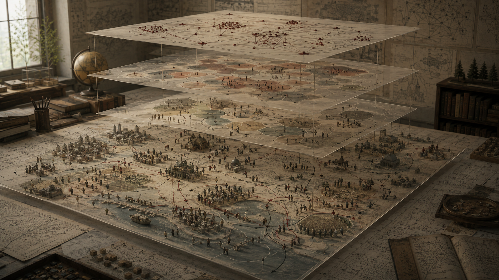
This article explains agent-based modeling as a major paradigm within systems modeling. It covers intellectual origins, agents and rules, environments, interaction structures, emergence, heterogeneity, adaptation, computational simulation, calibration, validation, uncertainty, policy use, sustainability applications, mathematical foundations, professional workflows, Python and R examples, strengths, limitations, and responsible interpretation.
What Is Agent-Based Modeling?
Agent-based modeling is a simulation method that represents a system as a population of interacting agents. Each agent is an entity with attributes, rules, state variables, and possible behaviors. Agents may represent people, firms, households, vehicles, organisms, institutions, infrastructure assets, technologies, or decision units. The model specifies how agents perceive information, make decisions, interact with others, adapt to conditions, and change the environment around them.
The key feature of ABM is that system-level behavior is not imposed from above. It emerges from the repeated operation of local rules. A modeler defines agents and interaction conditions, then observes how macro-level patterns develop over time. These patterns may include clustering, diffusion, congestion, segregation, cooperation, collapse, adaptation, contagion, adoption, polarization, inequality, resilience, or institutional change.
Agent-based modeling is especially useful when the system cannot be represented adequately by averages alone. If actors differ from one another, if local interaction matters, if network position shapes behavior, if adaptation changes future decisions, or if macro-patterns emerge from micro-level behavior, ABM may be appropriate.
| ABM element | Meaning | Why it matters |
|---|---|---|
| Agent | An individual entity with state, attributes, and behavior. | Represents heterogeneity and decentralized decision-making. |
| Rule | A formal decision or behavior rule. | Defines how agents act under different conditions. |
| Environment | The spatial, institutional, ecological, or network context. | Shapes what agents can observe, access, and change. |
| Interaction | A mechanism through which agents influence one another. | Produces diffusion, coordination, contagion, competition, or conflict. |
| Adaptation | Change in agent behavior over time. | Represents learning, imitation, selection, and response. |
| Emergence | System-level pattern generated by local interaction. | Explains macro behavior without assuming centralized control. |
ABM is therefore not simply a modeling technique for “many individuals.” It is a way to study how decentralized interaction produces system behavior.
Why Agent-Based Modeling Matters
Agent-based modeling matters because many complex systems are not governed by one average actor. They are composed of diverse agents operating under incomplete information, different incentives, unequal resources, bounded rationality, local relationships, and changing environments.
Traditional aggregate models can be powerful when the system can be represented through population-level quantities. But they may miss important mechanisms when heterogeneity and interaction matter. A public-health model may need to represent differences in contact patterns, mobility, risk perception, household structure, and access to care. A market model may need to represent firms with different strategies, capital, expectations, and network positions. An urban model may need to represent households with different preferences, income levels, commute patterns, and neighborhood constraints.
Agent-based modeling allows analysts to explore questions such as:
- How can mild local preferences generate strong aggregate segregation?
- How do innovations spread through social networks?
- How do local decisions create traffic congestion?
- How do heterogeneous firms generate market volatility?
- How does cooperation emerge under repeated interaction?
- How do policies affect different actors differently?
- How does adaptation change the effect of an intervention?
The value of ABM is not that it predicts every individual action precisely. Its value is that it provides a computational laboratory for testing how local rules, agent diversity, and interaction structures can generate plausible system-level outcomes.
Intellectual Origins
The intellectual roots of agent-based modeling lie in economics, political science, sociology, ecology, artificial intelligence, computer science, game theory, cellular automata, and complexity science. ABM developed as researchers began asking how macro-level patterns could emerge from micro-level behavior.
One of the most influential early examples was Thomas Schelling’s work on residential segregation. Schelling showed that strong aggregate segregation could emerge even when individual agents had only mild local preferences. This became a classic demonstration of the ABM logic: macro-level outcomes may be unintended consequences of local decisions.
Robert Axelrod’s computational work on cooperation also shaped the field. By simulating repeated interaction among strategies, Axelrod showed how cooperation could emerge under certain conditions without centralized control. This reinforced the idea that simulation could be used to study generative mechanisms in social systems.
Complexity science expanded the intellectual context for ABM. Research communities associated with the Santa Fe Institute helped popularize the study of complex adaptive systems, where many interacting agents adapt and co-evolve. Computational platforms such as NetLogo made agent-based modeling more accessible to researchers, students, and educators.
| Intellectual source | Contribution to ABM | Modeling significance |
|---|---|---|
| Schelling-style micro-macro modeling | Local preferences can generate unexpected aggregate patterns. | Shows why system outcomes may differ from individual intentions. |
| Repeated-game simulation | Strategies interact over time and produce cooperation or conflict. | Supports modeling of adaptation, reciprocity, and institutional behavior. |
| Cellular automata | Simple local update rules can generate complex spatial patterns. | Supports grid-based agent and environment models. |
| Complex adaptive systems | Agents adapt within dynamic environments. | Connects ABM to emergence, learning, and co-evolution. |
| Computational social science | Social mechanisms can be explored through simulation. | Supports generative explanation and scenario experimentation. |
ABM therefore emerged because many important systems required a modeling approach that could represent heterogeneity, interaction, adaptation, and emergence directly.
Agents, Rules, and Environments
An agent-based model begins by defining the agents. Each agent has attributes and state variables. These may include location, type, wealth, belief, health status, strategy, risk tolerance, capacity, memory, energy, preference, knowledge, or network position. The model then defines how agents update their state over time.
Rules may be simple or complex. An agent may move if dissatisfied with its neighborhood. A household may adopt a technology if enough neighbors have adopted. A firm may change price based on demand. A vehicle may slow down when nearby traffic is dense. A patient may seek care based on symptoms, access, and trust. A species may move toward resources and away from predators.
The environment matters because agents do not act in a vacuum. They act in space, networks, institutions, ecosystems, markets, or service systems. The environment may constrain movement, provide resources, transmit information, create hazards, store memory, or change in response to agent behavior.
| Design choice | Question | Example |
|---|---|---|
| Agent type | What entities are being modeled? | Households, firms, patients, vehicles, organisms, institutions. |
| Agent state | What changes within each agent? | Belief, health, adoption status, wealth, location, strategy. |
| Behavioral rule | How does the agent act? | Move, adopt, cooperate, compete, imitate, consume, invest. |
| Environment | Where do agents act? | Grid, network, market, city, landscape, organization, institution. |
| Interaction | How do agents affect one another? | Neighbor influence, contact, exchange, contagion, communication. |
| Outcome measure | What macro-pattern is observed? | Adoption rate, clustering, inequality, congestion, infection prevalence. |
A professional ABM must document these design choices clearly because they define what the model can and cannot explain.
Heterogeneity and Bounded Rationality
One of the main strengths of ABM is its ability to represent heterogeneity. Agents can differ in preferences, resources, thresholds, locations, information, risk perception, access, memory, social ties, institutional roles, and decision rules. This makes ABM useful for systems where averages conceal meaningful differences.
Heterogeneity matters because the same policy or shock can affect agents differently. A subsidy may be valuable to agents with enough capital to act on it but irrelevant to agents facing liquidity constraints. A public-health message may influence agents who trust institutions but fail among agents with different experiences or network influences. A technology may spread quickly through highly connected agents but stall in isolated groups.
ABM also allows bounded rationality. Agents do not need to optimize perfectly. They can use heuristics, imitate neighbors, respond to local information, follow habits, make mistakes, learn slowly, or adapt under constraints. This is often more realistic than assuming complete information and perfect optimization.
| Agent difference | Why it matters | Modeling example |
|---|---|---|
| Thresholds | Agents adopt or act under different conditions. | Some households adopt solar after one neighbor; others require many adopters. |
| Network position | Some agents influence or receive more information than others. | Central nodes accelerate diffusion. |
| Resources | Agents differ in capacity to respond. | Firms with higher reserves survive shocks longer. |
| Beliefs and trust | Agents interpret information differently. | Public-health compliance varies by trust and peer influence. |
| Location | Spatial exposure and access differ. | Flood risk, transit access, or service availability varies by neighborhood. |
By representing heterogeneity explicitly, ABM can reveal distributional effects and emergent patterns that aggregate models may flatten.
Interaction Structures
Agent behavior depends not only on individual rules, but also on who interacts with whom. Interaction structure determines how information, influence, disease, innovation, conflict, cooperation, risk, and resources move through the system.
Some ABMs use spatial neighborhoods. Agents interact with nearby agents on a grid or landscape. Others use networks. Agents interact through social ties, trade relationships, institutional links, infrastructure dependencies, or contact networks. Some models use well-mixed interaction, where any agent may interact with any other. Others use layered interaction, where agents interact differently across household, workplace, community, market, and digital networks.
| Interaction structure | Useful when | Example |
|---|---|---|
| Grid or lattice | Spatial proximity shapes behavior. | Segregation, land use, wildfire spread, ecological movement. |
| Social network | Influence and information move through relationships. | Technology adoption, norms, misinformation, cooperation. |
| Contact network | Transmission depends on encounters. | Infectious disease spread, mobility, exposure. |
| Market interaction | Agents exchange goods, services, labor, or capital. | Price dynamics, firm competition, labor markets. |
| Institutional setting | Rules and constraints shape agent behavior. | Policy compliance, permitting, governance, service access. |
Interaction structure is one of the most important ABM design choices. The same agents and rules may produce different macro-outcomes under different networks or environments.
Emergence and Complex Adaptive Systems
Emergence occurs when system-level behavior arises from interactions among lower-level components. In ABM, emergence is not merely a metaphor. It is a modeling object. The analyst specifies agent rules and interaction conditions, then observes macro-patterns generated by those micro-processes.
Examples of emergent behavior include residential segregation, market bubbles, traffic jams, cooperation, polarization, disease waves, clustering, resource depletion, institutional norms, and technology diffusion. In each case, the macro-pattern cannot be fully understood by examining one isolated actor. It depends on repeated interaction across many agents.
Complex adaptive systems add another layer: agents adapt. They learn, imitate, switch strategies, respond to payoffs, change locations, update beliefs, or modify networks. This can create co-evolution between agents and environments. A city shapes mobility choices, but mobility choices also shape the city. A market shapes firm behavior, but firm behavior reshapes market conditions. An institution shapes incentives, but agents adapt to institutional rules in ways that may reinforce or undermine those rules.
\text{Local Rules}+\text{Interaction Structure}+\text{Adaptation}\rightarrow \text{Emergent System Behavior}
\]
Interpretation: ABM studies how macro-level patterns arise from repeated micro-level interactions among agents embedded in environments.
This is why ABM is central to complexity science. It provides a computational method for exploring how decentralized behavior can produce organized, unstable, adaptive, or unexpected system outcomes.
Adaptation, Learning, and Path Dependence
Many systems change because agents learn from experience. Agents may adjust behavior after success or failure. They may imitate successful neighbors. They may update expectations. They may become more cautious after shocks. They may abandon strategies that no longer work. They may change their relationships or locations.
ABM can represent adaptation through rule updates, reinforcement learning, evolutionary selection, imitation, memory, or institutional feedback. These mechanisms matter because the effect of a policy may change as agents respond to it. A regulation may create compliance, evasion, innovation, backlash, or new strategic behavior. A subsidy may encourage adoption, but adoption may later become self-reinforcing through peer effects.
Path dependence occurs when early events shape later possibilities. Initial adopters may determine the direction of a technology market. Early settlement patterns may shape long-term urban structure. Early trust failures may constrain later public cooperation. Initial network positions may produce durable inequality.
| Adaptive mechanism | Meaning | Example |
|---|---|---|
| Imitation | Agents copy successful or nearby agents. | Farmers adopt practices used by trusted neighbors. |
| Learning | Agents update beliefs based on experience. | Firms adjust strategies after repeated losses. |
| Selection | Some strategies survive while others disappear. | Market competition eliminates weak business models. |
| Memory | Past experience shapes future behavior. | Communities distrust institutions after repeated failures. |
| Network rewiring | Agents change relationships over time. | People leave low-value networks and join more useful ones. |
Adaptation makes ABM especially valuable for policy analysis because policy does not act on passive systems. It acts on agents who interpret, respond, and adapt.
ABM vs Aggregate Modeling
Agent-based modeling differs from aggregate modeling in both starting point and explanatory logic. Aggregate models usually represent systems through population-level variables: total demand, average income, infection prevalence, mean behavior, total emissions, or representative firms. These models can be powerful, especially when aggregate quantities are the right level of analysis.
ABM begins at the level of agents. It asks how aggregate quantities arise from individual behavior and interaction. Instead of assuming a representative actor, ABM can represent many actors with different attributes, thresholds, rules, and network positions.
| Dimension | Aggregate modeling | Agent-based modeling |
|---|---|---|
| Starting point | Population-level variables. | Individual agents and local rules. |
| Behavior | Often averaged or representative. | Heterogeneous, bounded, adaptive, rule-based. |
| Interaction | Often implicit or aggregated. | Explicit local, spatial, networked, or institutional interaction. |
| Macro outcomes | Specified through equations. | Generated from micro-level simulation. |
| Best suited for | Aggregate dynamics, stock-flow systems, equilibrium or macro trends. | Emergence, diffusion, heterogeneity, adaptation, local interaction. |
ABM does not replace aggregate modeling. It complements it. Many professional systems models combine ABM with system dynamics, network models, discrete-event simulation, or statistical models. The correct method depends on the structure of the problem.
Computational Simulation
Agent-based models are implemented as simulations because the behavior of many interacting agents is often difficult to solve analytically. The model runs through repeated time steps. At each step, agents observe conditions, update states, interact, move, decide, learn, or modify the environment. The model records system-level outcomes after each step.
Many ABMs are stochastic. Randomness may appear in initial conditions, movement, interaction, decisions, shocks, or adaptation. This means a single run may not be enough. Analysts often run ensembles: many repeated simulations under the same or varied assumptions. The distribution of outcomes can then be analyzed.
Simulation outputs may include trajectories, spatial maps, network metrics, adoption curves, inequality measures, infection curves, clustering indices, resilience measures, or policy performance indicators. Because ABM can generate large volumes of output, professional practice requires careful diagnostics, version control, documentation, and reproducibility.
| Simulation concern | Why it matters | Professional practice |
|---|---|---|
| Initialization | Early conditions may shape later patterns. | Document initial states and test alternative starts. |
| Randomness | Single runs may be misleading. | Use repeated runs and report distributions. |
| Scheduling | Order of agent updates can affect outcomes. | Specify synchronous, asynchronous, random, or staged updates. |
| Scalability | Large agent populations can be computationally expensive. | Profile performance and simplify where appropriate. |
| Output interpretation | Complex outputs can be difficult to summarize. | Use clear diagnostics and scenario comparisons. |
A good ABM workflow treats simulation as an experiment. It defines assumptions, runs the model systematically, analyzes outputs, and reports uncertainty.
Calibration, Validation, and Credibility
Calibration and validation are challenging in agent-based modeling because ABMs often contain many assumptions about behavior, interaction, adaptation, and environment. Calibration may involve matching model parameters to data, known distributions, expert judgment, or observed patterns. Validation evaluates whether the model is credible for its intended purpose.
ABM validation should consider both micro-level and macro-level credibility. Are the agent rules plausible? Are the interaction structures realistic? Do the outputs reproduce relevant patterns? Are results robust across parameter ranges? Does the model behave plausibly under extreme conditions? Are the assumptions transparent enough to critique?
The ODD protocol, short for Overview, Design concepts, and Details, is widely used to document agent-based and individual-based models. It helps modelers describe purpose, entities, state variables, process overview, scheduling, design concepts, initialization, inputs, and submodels.
| Credibility question | ABM concern | Example check |
|---|---|---|
| Micro-level validity | Are agent rules plausible? | Compare rules with empirical studies, interviews, or domain expertise. |
| Interaction validity | Are relationships represented appropriately? | Test alternative networks, neighborhoods, or contact structures. |
| Macro-level validity | Does the model reproduce relevant system patterns? | Compare adoption curves, clustering, congestion, or spread patterns. |
| Sensitivity | Which assumptions drive outcomes? | Vary thresholds, network density, behavioral rules, and initial states. |
| Reproducibility | Can others inspect and rerun the model? | Publish code, seeds, data, documentation, and run instructions. |
Credibility is purpose-specific. A teaching model, exploratory mechanism model, policy-support model, and operational decision model require different evidence standards.
Software Tools for Agent-Based Modeling
Agent-based modeling can be built in specialized simulation platforms or general-purpose programming languages. The right tool depends on the model’s purpose, scale, audience, visualization needs, reproducibility requirements, and integration with other workflows.
NetLogo is widely used in research and education because it makes multi-agent modeling accessible. Mesa supports agent-based modeling in Python and is useful for reproducible research workflows. Repast, AnyLogic, GAMA, MASON, and other platforms support more specialized or large-scale modeling needs. Some professional teams build custom ABMs in Python, R, Julia, Java, C++, Rust, or other languages when performance, integration, or transparency requires it.
| Tool | Common use | Modeling caution |
|---|---|---|
| NetLogo | Education, research prototypes, visual ABM, model libraries. | Useful for learning and communication, but large models may require performance planning. |
| Mesa | Python-based ABM, reproducible workflows, integration with data analysis. | Requires careful software organization and documentation. |
| Repast | Research-oriented agent simulation frameworks. | More technical setup may be required. |
| AnyLogic | Commercial hybrid simulation with ABM, system dynamics, and discrete events. | Licensing and transparency considerations may matter. |
| Custom code | High-control, reproducible, domain-specific simulation. | Requires testing, validation, and maintainable architecture. |
Software choice does not determine model quality. The quality of an ABM depends on assumptions, structure, evidence, diagnostics, documentation, and interpretation.
Applications Across Complex Systems
Urban systems
Households, commuters, developers, firms, and institutions interact through housing, mobility, land use, infrastructure, and neighborhood change.
Epidemiology
Individuals differ in contacts, mobility, susceptibility, behavior, risk perception, and access to care, shaping disease spread and intervention effects.
Economics and markets
Firms, households, investors, workers, and institutions interact through bounded rationality, expectations, competition, and adaptation.
Ecology
Organisms move, reproduce, compete, forage, disperse, and adapt within spatial environments and changing ecological constraints.
Transportation
Drivers, vehicles, pedestrians, transit users, and logistics operators create congestion, route choice patterns, and network effects.
Organizations
Workers, teams, managers, and institutions interact through workload, coordination, trust, incentives, learning, and turnover.
Technology adoption
Adoption spreads through networks, peer influence, price, learning, infrastructure, trust, and institutional support.
Public policy
Policies affect agents differently, and agents adapt through compliance, evasion, learning, cooperation, or resistance.
Across these applications, ABM is valuable when the behavior of the whole system depends on the interaction of diverse parts.
Applications in Sustainability and Policy
Agent-based modeling is especially important for sustainability and public policy because transitions depend on heterogeneous behavior. Energy adoption, land-use change, mobility behavior, water use, conservation practices, food systems, disaster response, climate adaptation, and institutional trust all involve agents who differ in resources, incentives, beliefs, constraints, and network positions.
A policy rarely affects all agents equally. A subsidy may accelerate adoption among high-resource agents while leaving low-resource agents behind. A climate adaptation program may work in communities with strong institutions but fail where trust is low. A transportation intervention may change mobility behavior differently across income, geography, disability status, and service access.
ABM can help policy analysts examine distributional and behavioral effects that aggregate models may miss. It can test how interventions diffuse, how adoption thresholds vary, how network position affects access, how institutional constraints shape behavior, and how unintended consequences arise through adaptation.
| Policy area | ABM contribution | Possible output |
|---|---|---|
| Energy transition | Models heterogeneous technology adoption and peer effects. | Adoption curves, equity gaps, diffusion clusters. |
| Climate adaptation | Represents household, firm, and institutional response to risk. | Preparedness, migration, investment, vulnerability. |
| Urban planning | Models location choice, mobility, housing, and neighborhood dynamics. | Congestion, segregation, displacement, accessibility. |
| Public health | Models contact patterns and behavioral response. | Infection trajectories, intervention uptake, care demand. |
| Environmental governance | Models cooperation, compliance, monitoring, and enforcement. | Resource use, cooperation rates, institutional resilience. |
ABM does not make policy decisions by itself. It helps decision-makers examine how policies may unfold when real actors respond unevenly and adaptively.
Mathematical Lens: Local Rules, State Transitions, and Emergence
A simple agent-based model can be expressed through agent states and update rules. Let agent \(i\) have state \(s_i(t)\) at time \(t\). The agent’s next state may depend on its current state, neighbors, environment, parameters, and random variation:
s_i(t+1)=F_i\left(s_i(t),\mathcal{N}_i(t),E(t),\theta_i,\varepsilon_i(t)\right)
\]
Interpretation: Agent \(i\)’s next state depends on its current condition, local neighborhood, environment, parameters, and uncertainty.
The neighborhood \(\mathcal{N}_i(t)\) may be spatial, social, institutional, or network-based:
\mathcal{N}_i(t)=\{j:A_{ij}(t)>0\}
\]
Interpretation: Agent \(i\)’s neighbors are agents connected to it through an adjacency structure \(A\).
A macro-level observable can be calculated from all agent states:
M(t)=G\left(s_1(t),s_2(t),\ldots,s_n(t)\right)
\]
Interpretation: The system-level pattern \(M(t)\) emerges from the collection of agent states.
For adoption modeling, a threshold rule might be written as:
s_i(t+1)=
\begin{cases}
1, & \text{if } \frac{1}{|\mathcal{N}_i|}\sum_{j\in \mathcal{N}_i}s_j(t)\geq \tau_i \\
s_i(t), & \text{otherwise}
\end{cases}
\]
Interpretation: Agent \(i\) adopts when the share of adopting neighbors exceeds its individual threshold \(\tau_i\).
This mathematical lens captures the core ABM idea: the model is specified at the micro level, but the analytical interest often lies in macro-level patterns generated by repeated decentralized interaction.
The Agent-Based Modeling Workflow
Professional ABM requires more than writing agents into code. It requires disciplined model purpose, boundary setting, rule design, calibration, sensitivity testing, validation, documentation, and interpretation.
1. Define the behavior of interest
Start with the system-level pattern the model is meant to explain or explore: diffusion, clustering, segregation, cooperation, congestion, disease spread, market instability, adoption, or resilience.
2. Establish the model boundary
Decide which agents, environments, institutions, networks, resources, and external drivers are included. Document what remains outside the model.
3. Specify agent types and state variables
Define the agents, their attributes, their changing states, and the differences among them. Heterogeneity should serve the modeling purpose.
4. Define behavioral rules
Translate assumptions about decision-making into explicit rules. Rules may include thresholds, heuristics, optimization, imitation, learning, or institutional constraints.
5. Define interaction structure
Specify whether agents interact through space, networks, markets, institutions, events, or random contact. Interaction structure often drives model outcomes.
6. Specify scheduling and time
Decide whether agents update synchronously, asynchronously, randomly, sequentially, or through staged processes. Scheduling can change results.
7. Run baseline simulations
Test whether the model generates plausible behavior under reference assumptions. Record seeds, parameters, outputs, and diagnostics.
8. Compare scenarios and ensembles
Run repeated simulations across parameter ranges, initial conditions, network structures, policies, and shocks. ABM results should rarely rely on one run.
9. Validate for purpose
Assess micro-level rule plausibility, macro-level pattern reproduction, sensitivity, robustness, documentation quality, and stakeholder credibility.
10. Communicate responsibly
Explain assumptions, uncertainty, calibration limits, scenario design, and appropriate use. ABM should support learning, not create false certainty.
Strengths and Limitations
Agent-based modeling is powerful because it can represent heterogeneous agents, local interaction, emergence, adaptation, and path dependence. It can show how system-level outcomes arise even when no agent intends them. It can reveal distributional effects that aggregate models may hide. It can test behavioral assumptions under different scenarios.
At the same time, ABM has limitations. Agent rules can be difficult to justify. Models may contain many parameters. Results may be sensitive to initial conditions, randomness, update schedules, or network assumptions. Complex ABMs can become opaque. Calibration and validation may be difficult when data are limited. Computational cost can rise quickly as agent populations and interaction structures grow.
| Strength | Why it matters | Limitation to watch |
|---|---|---|
| Represents heterogeneity | Captures differences among agents. | Too much detail can make the model hard to interpret. |
| Represents local interaction | Shows how neighborhoods and networks shape outcomes. | Interaction assumptions may dominate results. |
| Generates emergence | Explains macro patterns from micro rules. | Emergent patterns may be hard to validate. |
| Supports adaptation | Models learning, imitation, and strategic response. | Adaptive rules require strong justification. |
| Supports scenario testing | Explores policy and uncertainty. | Single-run outputs can be misleading. |
The best ABMs are not necessarily the most detailed. They are the ones whose agents, rules, interactions, and outputs are appropriate for the question being asked.
Python Workflow: Schelling-Style Clustering and Emergence
The Python workflow below uses only the standard library. It simulates a Schelling-style spatial model in which agents move when local neighborhood composition falls below their satisfaction threshold. It writes reproducible outputs for trajectories, summary metrics, and final grid state.
# agent_based_modeling_workflow.py
# Dependency-light ABM workflow:
# Schelling-style local interaction, movement, clustering, and emergence.
#
# Suggested repository placement:
# articles/agent-based-modeling/python/agent_based_modeling_workflow.py

from __future__ import annotations

from dataclasses import dataclass
from pathlib import Path
import csv
import random
from statistics import mean


ARTICLE_ROOT = Path(__file__).resolve().parents[1]
TABLES = ARTICLE_ROOT / "outputs" / "tables"


@dataclass(frozen=True)
class Scenario:
    name: str
    grid_size: int = 24
    empty_share: float = 0.18
    type_a_share: float = 0.41
    satisfaction_threshold: float = 0.45
    max_steps: int = 60
    seed: int = 4201


def write_csv(path: Path, rows: list[dict[str, object]]) -> None:
    path.parent.mkdir(parents=True, exist_ok=True)
    if not rows:
        raise ValueError(f"No rows to write: {path}")
    with path.open("w", newline="", encoding="utf-8") as handle:
        writer = csv.DictWriter(handle, fieldnames=list(rows[0].keys()))
        writer.writeheader()
        writer.writerows(rows)


def initialize_grid(scenario: Scenario) -> list[list[int]]:
    rng = random.Random(scenario.seed)
    grid: list[list[int]] = []

    for _ in range(scenario.grid_size):
        row = []
        for _ in range(scenario.grid_size):
            draw = rng.random()
            if draw < scenario.empty_share:
                row.append(-1)
            elif draw < scenario.empty_share + scenario.type_a_share: row.append(0) else: row.append(1) grid.append(row) return grid def neighbors(grid: list[list[int]], row: int, col: int) -> list[int]:
    n = len(grid)
    values: list[int] = []

    for dr in [-1, 0, 1]:
        for dc in [-1, 0, 1]:
            if dr == 0 and dc == 0:
                continue
            rr = row + dr
            cc = col + dc
            if 0 <= rr < n and 0 <= cc < n and grid[rr][cc] != -1: values.append(grid[rr][cc]) return values def same_share(grid: list[list[int]], row: int, col: int) -> float:
    agent_type = grid[row][col]
    if agent_type == -1:
        return 1.0

    local = neighbors(grid, row, col)
    if not local:
        return 1.0

    return sum(1 for value in local if value == agent_type) / len(local)


def empty_cells(grid: list[list[int]]) -> list[tuple[int, int]]:
    cells = []
    for row in range(len(grid)):
        for col in range(len(grid[row])):
            if grid[row][col] == -1:
                cells.append((row, col))
    return cells


def occupied_cells(grid: list[list[int]]) -> list[tuple[int, int]]:
    cells = []
    for row in range(len(grid)):
        for col in range(len(grid[row])):
            if grid[row][col] != -1:
                cells.append((row, col))
    return cells


def clustering_index(grid: list[list[int]]) -> float:
    shares = []
    for row, col in occupied_cells(grid):
        shares.append(same_share(grid, row, col))
    return mean(shares) if shares else 0.0


def simulate(scenario: Scenario) -> tuple[list[dict[str, object]], list[dict[str, object]]]:
    rng = random.Random(scenario.seed + 1000)
    grid = initialize_grid(scenario)

    trajectory: list[dict[str, object]] = []

    for step in range(scenario.max_steps + 1):
        occupied = occupied_cells(grid)
        unhappy = [
            (row, col)
            for row, col in occupied
            if same_share(grid, row, col) < scenario.satisfaction_threshold ] satisfied_share = 1.0 - (len(unhappy) / len(occupied) if occupied else 0.0) trajectory.append({ "scenario": scenario.name, "step": step, "occupied_agents": len(occupied), "unhappy_agents": len(unhappy), "satisfied_share": round(satisfied_share, 6), "clustering_index": round(clustering_index(grid), 6), "empty_cells": len(empty_cells(grid)), }) if not unhappy: break vacancies = empty_cells(grid) rng.shuffle(unhappy) rng.shuffle(vacancies) for row, col in unhappy: if not vacancies: break new_row, new_col = vacancies.pop() grid[new_row][new_col] = grid[row][col] grid[row][col] = -1 vacancies.append((row, col)) final_grid_rows: list[dict[str, object]] = [] for row in range(len(grid)): for col in range(len(grid[row])): final_grid_rows.append({ "scenario": scenario.name, "row": row, "col": col, "agent_type": grid[row][col], }) return trajectory, final_grid_rows def summarize(trajectory: list[dict[str, object]]) -> dict[str, object]:
    first = trajectory[0]
    last = trajectory[-1]

    return {
        "scenario": last["scenario"],
        "steps_completed": last["step"],
        "initial_satisfied_share": first["satisfied_share"],
        "final_satisfied_share": last["satisfied_share"],
        "initial_clustering_index": first["clustering_index"],
        "final_clustering_index": last["clustering_index"],
        "final_unhappy_agents": last["unhappy_agents"],
        "diagnostic": (
            "local preferences generated stronger clustering"
            if float(last["clustering_index"]) > float(first["clustering_index"])
            else "limited clustering change under current assumptions"
        ),
    }


def main() -> None:
    scenarios = [
        Scenario(name="baseline_abm"),
        Scenario(name="low_threshold", satisfaction_threshold=0.30, seed=4202),
        Scenario(name="high_threshold", satisfaction_threshold=0.60, seed=4203),
        Scenario(name="fewer_empty_cells", empty_share=0.10, seed=4204),
        Scenario(name="more_empty_cells", empty_share=0.28, seed=4205),
    ]

    all_trajectories: list[dict[str, object]] = []
    all_grids: list[dict[str, object]] = []
    summaries: list[dict[str, object]] = []

    for scenario in scenarios:
        trajectory, grid_rows = simulate(scenario)
        all_trajectories.extend(trajectory)
        all_grids.extend(grid_rows)
        summaries.append(summarize(trajectory))

    write_csv(TABLES / "python_abm_schelling_trajectory.csv", all_trajectories)
    write_csv(TABLES / "python_abm_schelling_final_grid.csv", all_grids)
    write_csv(TABLES / "python_abm_schelling_summary.csv", summaries)

    print("Agent-based modeling workflow complete.")
    print(TABLES / "python_abm_schelling_summary.csv")


if __name__ == "__main__":
    main()
This workflow demonstrates the ABM logic: local rules can generate macro-level clustering. The model does not assume segregation or clustering as an output. It emerges from repeated local decisions under different threshold and vacancy assumptions.
R Workflow: Threshold Adoption with Heterogeneous Agents
The R workflow below uses base R. It simulates heterogeneous agents on a ring network. Each agent has an adoption threshold and adopts when local adoption among neighbors crosses that threshold. The workflow writes adoption trajectories and scenario summaries.
# agent_based_modeling_diagnostics.R
# Base R workflow:
# threshold adoption with heterogeneous agents and local network influence.
#
# Suggested repository placement:
# articles/agent-based-modeling/r/agent_based_modeling_diagnostics.R

args <- commandArgs(trailingOnly = FALSE)
file_arg <- grep("^--file=", args, value = TRUE) if (length(file_arg) > 0) {
  script_path <- normalizePath(sub("^--file=", "", file_arg[1]), mustWork = TRUE)
  article_root <- normalizePath(file.path(dirname(script_path), ".."), mustWork = TRUE)
} else {
  article_root <- normalizePath(getwd(), mustWork = TRUE)
}

tables_dir <- file.path(article_root, "outputs", "tables")
figures_dir <- file.path(article_root, "outputs", "figures")

dir.create(tables_dir, recursive = TRUE, showWarnings = FALSE)
dir.create(figures_dir, recursive = TRUE, showWarnings = FALSE)

simulate_threshold_adoption <- function(
  scenario,
  n_agents = 180,
  n_steps = 50,
  initial_adopters = 12,
  threshold_low = 0.10,
  threshold_high = 0.70,
  neighbor_radius = 2,
  seed = 101
) {
  set.seed(seed)

  thresholds <- runif(n_agents, threshold_low, threshold_high)
  adopted <- rep(FALSE, n_agents)
  adopted[sample(seq_len(n_agents), initial_adopters)] <- TRUE

  trajectory <- data.frame()

  for (time in seq_len(n_steps)) {
    previous <- adopted

    for (i in seq_len(n_agents)) {
      if (!previous[i]) {
        neighbor_ids <- c()

        for (offset in seq(-neighbor_radius, neighbor_radius)) {
          if (offset != 0) {
            neighbor <- ((i - 1 + offset) %% n_agents) + 1
            neighbor_ids <- c(neighbor_ids, neighbor)
          }
        }

        local_adoption_share <- mean(previous[neighbor_ids]) if (local_adoption_share >= thresholds[i]) {
          adopted[i] <- TRUE
        }
      }
    }

    trajectory <- rbind(trajectory, data.frame(
      scenario = scenario,
      time = time,
      adoption_rate = mean(adopted),
      new_adopters = sum(adopted) - sum(previous),
      mean_threshold = mean(thresholds),
      threshold_low = threshold_low,
      threshold_high = threshold_high,
      neighbor_radius = neighbor_radius
    ))
  }

  trajectory
}

all_data <- rbind(
  simulate_threshold_adoption("baseline_threshold_adoption", seed = 101),
  simulate_threshold_adoption("low_threshold_population", threshold_low = 0.05, threshold_high = 0.45, seed = 102),
  simulate_threshold_adoption("high_threshold_population", threshold_low = 0.35, threshold_high = 0.85, seed = 103),
  simulate_threshold_adoption("wider_neighborhood", neighbor_radius = 4, seed = 104),
  simulate_threshold_adoption("more_initial_adopters", initial_adopters = 28, seed = 105)
)

scenario_names <- unique(all_data$scenario)
summary_rows <- data.frame()

 for (scenario_name in scenario_names) {
  subset_data <- all_data[all_data$scenario == scenario_name, ]

  summary_rows <- rbind(summary_rows, data.frame( scenario = scenario_name, initial_adoption_rate = subset_data$adoption_rate[1], final_adoption_rate = tail(subset_data$adoption_rate, 1), peak_new_adopters = max(subset_data$new_adopters), time_to_half_adoption = ifelse( any(subset_data$adoption_rate >= 0.5),
      min(subset_data$time[subset_data$adoption_rate >= 0.5]),
      NA
    ),
    mean_threshold = unique(subset_data$mean_threshold)[1],
    diagnostic = ifelse(
      tail(subset_data$adoption_rate, 1) >= 0.8,
      "broad adoption emerged from local threshold dynamics",
      ifelse(
        tail(subset_data$adoption_rate, 1) >= 0.4,
        "partial adoption emerged under current assumptions",
        "adoption stalled under current assumptions"
      )
    )
  ))
}

write.csv(all_data, file.path(tables_dir, "r_abm_threshold_adoption_trajectory.csv"), row.names = FALSE)
write.csv(summary_rows, file.path(tables_dir, "r_abm_threshold_adoption_summary.csv"), row.names = FALSE)

png(file.path(figures_dir, "r_abm_threshold_adoption_trajectories.png"), width = 1200, height = 700)
plot(
  NA,
  xlim = range(all_data$time),
  ylim = c(0, 1),
  xlab = "Time",
  ylab = "Adoption Rate",
  main = "Threshold Adoption Across Heterogeneous Agent Scenarios"
)

for (scenario_name in scenario_names) {
  subset_data <- all_data[all_data$scenario == scenario_name, ]
  lines(subset_data$time, subset_data$adoption_rate, lwd = 2)
}

legend("bottomright", legend = scenario_names, lwd = 2, bty = "n", cex = 0.75)
grid()
dev.off()

print(summary_rows)
cat("R agent-based modeling diagnostics complete.\n")
This R workflow shows how adoption can spread through local influence even when agents differ in thresholds. The macro-level adoption curve emerges from heterogeneous local rules rather than from one aggregate adoption equation.
GitHub Repository
Complete Code Repository
Companion repository for the article, including Schelling-style clustering simulations, threshold-adoption models, heterogeneous-agent workflows, local interaction diagnostics, emergence measures, scenario comparisons, sensitivity checks, synthetic datasets, documentation assets, and multi-language examples for professional systems modeling.
Ethics and Responsible Use
Agent-based models can influence how institutions understand people, communities, markets, ecosystems, and public behavior. This gives ABM ethical significance. The modeler decides which agents exist, what rules they follow, what information they see, what constraints they face, and which outcomes matter. Those choices can clarify a system, but they can also encode bias, stereotype behavior, or hide structural power.
ABM is especially sensitive because it often represents people. A model of households, patients, migrants, neighborhoods, workers, or communities can easily simplify lived experience into rules that appear objective. Responsible ABM requires careful attention to data quality, behavioral assumptions, stakeholder knowledge, uncertainty, privacy, and interpretation.
| Responsible-use issue | Risk | Better practice |
|---|---|---|
| Behavioral simplification | Agents are assigned unrealistic or biased rules. | Ground rules in evidence, theory, domain expertise, and stakeholder review. |
| False realism | Detailed simulations appear more accurate than they are. | Report uncertainty, assumptions, and limits clearly. |
| Privacy and surveillance | Individual-level modeling can create sensitive data risks. | Use synthetic data, aggregation, minimization, and privacy safeguards. |
| Distributional blind spots | Model outputs hide unequal effects across groups. | Report subgroup outcomes and equity-relevant diagnostics. |
| Technocratic misuse | The model replaces democratic judgment. | Use ABM as a learning tool, not a final authority. |
A responsible ABM should make assumptions visible and contestable. It should improve understanding without pretending to fully capture human complexity.
Common Pitfalls
Agent-based modeling can fail when model detail grows faster than model discipline. More agents, more rules, and more outputs do not automatically produce better analysis. The model must remain aligned with its purpose.
| Pitfall | Why it matters | Correction |
|---|---|---|
| Overcomplicated agents | Too much behavioral detail can make the model opaque. | Include only complexity needed for the question. |
| Weak rule justification | Outputs depend on arbitrary behavior assumptions. | Document empirical, theoretical, or stakeholder basis for rules. |
| Single-run interpretation | Randomness can make one run misleading. | Use repeated runs, seeds, and output distributions. |
| Ignoring scheduling effects | Update order can change model behavior. | Specify and test scheduling assumptions. |
| Poor validation | Emergent patterns may be treated as credible without evidence. | Use pattern validation, sensitivity analysis, and expert review. |
| Confusing explanation with prediction | Generative models may be overused as forecasts. | Clarify whether the model is exploratory, explanatory, or predictive. |
Strong ABM practice requires transparency, sensitivity testing, documentation, and humility about what the model can show.
Conclusion
Agent-based modeling is one of the most important methods in systems modeling because it shows how macro-level patterns can emerge from micro-level interaction. By representing heterogeneous agents, local rules, environments, networks, adaptation, and decentralized decision-making, ABM makes complex adaptive behavior analyzable in a way that aggregate models often cannot.
ABM is especially valuable when system behavior depends on diversity, interaction, path dependence, learning, local information, or network position. It helps explain why neighborhoods cluster, technologies diffuse, markets fluctuate, diseases spread, institutions adapt, and policies produce uneven effects.
But agent-based modeling also requires caution. Its outputs depend on agent rules, interaction structures, initial conditions, random processes, and validation choices. A convincing simulation is not automatically a credible model. The value of ABM depends on clear purpose, transparent assumptions, careful diagnostics, repeated runs, sensitivity analysis, and responsible interpretation.
Used well, ABM is not a black box. It is a structured computational laboratory for studying how decentralized action produces complex system behavior.
Related Articles
- What Is Systems Modeling?
- Systems Thinking vs Systems Modeling
- Why Complex Systems Require Models
- The History of Systems Modeling
- Core Principles of Systems Modeling
- System Dynamics Modeling
- Network Models
- Hybrid Modeling Approaches
- Calibration and Validation of Models
Further Reading
- NetLogo. NetLogo Home. Available at: https://www.netlogo.org/.
- Northwestern Center for Connected Learning. NetLogo Models Library. Available at: https://ccl.northwestern.edu/netlogo/models/.
- Mesa. Agent-Based Modeling in Python. Available at: https://mesa.readthedocs.io/.
- Santa Fe Institute. Learn Agent-Based Modeling. Available at: https://www.santafe.edu/news-center/news/learn-agent-based-modeling.
- Santa Fe Institute. What is Complex Systems Science? Available at: https://www.santafe.edu/what-is-complex-systems-science.
- Grimm, V. et al. (2020) The ODD Protocol for Describing Agent-Based and Other Simulation Models: A Second Update to Improve Clarity, Replication, and Structural Realism. Available at: https://www.jasss.org/23/2/7.html.
- Axelrod, R. (1984) The Evolution of Cooperation. New York: Basic Books.
- Axelrod, R. (1997) The Complexity of Cooperation: Agent-Based Models of Competition and Collaboration. Princeton: Princeton University Press.
- Epstein, J.M. (2006) Generative Social Science: Studies in Agent-Based Computational Modeling. Princeton: Princeton University Press.
- Epstein, J.M. and Axtell, R. (1996) Growing Artificial Societies: Social Science from the Bottom Up. Washington, DC: Brookings Institution Press.
- Gilbert, N. (2008) Agent-Based Models. Thousand Oaks, CA: SAGE Publications.
- Railsback, S.F. and Grimm, V. (2019) Agent-Based and Individual-Based Modeling: A Practical Introduction. Princeton: Princeton University Press.
- Schelling, T.C. (1978) Micromotives and Macrobehavior. New York: W.W. Norton.
- Wilensky, U. and Rand, W. (2015) An Introduction to Agent-Based Modeling: Modeling Natural, Social, and Engineered Complex Systems with NetLogo. Cambridge, MA: MIT Press.
References
- Axelrod, R. (1984) The Evolution of Cooperation. New York: Basic Books.
- Axelrod, R. (1997) The Complexity of Cooperation: Agent-Based Models of Competition and Collaboration. Princeton: Princeton University Press.
- Epstein, J.M. (2006) Generative Social Science: Studies in Agent-Based Computational Modeling. Princeton: Princeton University Press.
- Epstein, J.M. and Axtell, R. (1996) Growing Artificial Societies: Social Science from the Bottom Up. Washington, DC: Brookings Institution Press.
- Gilbert, N. (2008) Agent-Based Models. Thousand Oaks, CA: SAGE Publications.
- Grimm, V. et al. (2020) The ODD Protocol for Describing Agent-Based and Other Simulation Models: A Second Update to Improve Clarity, Replication, and Structural Realism. Journal of Artificial Societies and Social Simulation, 23(2), 7. Available at: https://www.jasss.org/23/2/7.html.
- Mesa. (n.d.) Agent-Based Modeling in Python. Available at: https://mesa.readthedocs.io/.
- NetLogo. (n.d.) NetLogo Home. Available at: https://www.netlogo.org/.
- Northwestern Center for Connected Learning. (n.d.) NetLogo Models Library. Available at: https://ccl.northwestern.edu/netlogo/models/.
- Railsback, S.F. and Grimm, V. (2019) Agent-Based and Individual-Based Modeling: A Practical Introduction. Princeton: Princeton University Press.
- Santa Fe Institute. (2019) Learn Agent-Based Modeling. Available at: https://www.santafe.edu/news-center/news/learn-agent-based-modeling.
- Schelling, T.C. (1978) Micromotives and Macrobehavior. New York: W.W. Norton.
- Wilensky, U. (1999) NetLogo. Center for Connected Learning and Computer-Based Modeling, Northwestern University. Available at: https://www.netlogo.org/.
- Wilensky, U. and Rand, W. (2015) An Introduction to Agent-Based Modeling: Modeling Natural, Social, and Engineered Complex Systems with NetLogo. Cambridge, MA: MIT Press.