
Last Updated June 20, 2026
Search spaces and computational exploration explain how algorithms move through possible states, solutions, paths, hypotheses, configurations, assignments, plans, explanations, and decisions. Many computational problems are not solved by applying a single formula directly. They are solved by exploring a space of possibilities and deciding which possibilities are worth expanding, pruning, ranking, testing, or rejecting.
A search space is the structured set of possible states or candidate answers that a computational process may consider. In a maze, the search space includes possible locations and paths. In a scheduling problem, it includes possible assignments of people, rooms, tasks, and times. In diagnosis, it includes possible explanations for observed symptoms or failures. In planning, it includes possible sequences of actions. In optimization, it includes feasible solutions and trade-offs. In artificial intelligence, it may include hypotheses, moves, prompts, tool calls, model states, or chains of reasoning.
Computational exploration is the process of navigating that space. It asks where to begin, what to examine next, how to avoid repetition, how to recognize progress, how to detect dead ends, how to use heuristics, how to balance breadth and depth, how to stop, and how to explain what was searched and what was ignored.
This article introduces search spaces and computational exploration as core topics in algorithms and computational reasoning. It emphasizes that search is not only a technical procedure. It is a way of structuring uncertainty, possibility, constraint, evidence, and decision-making.
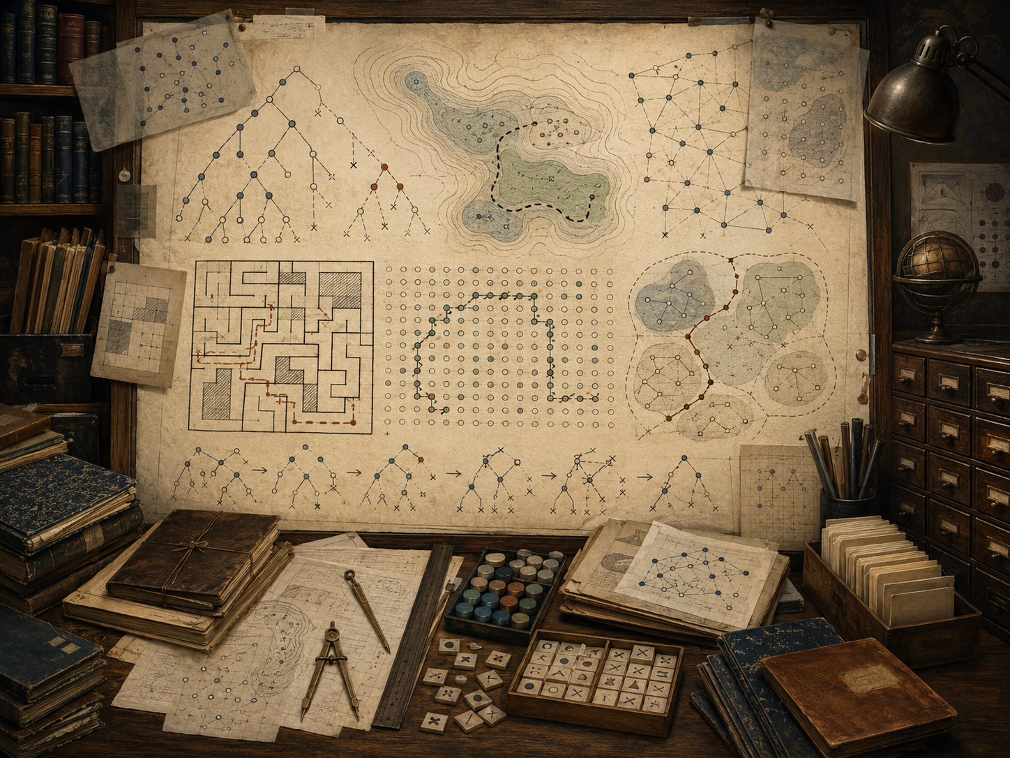
This article explains search spaces, states, transitions, initial states, goal states, candidate solutions, branching factors, frontiers, explored sets, path cost, heuristics, pruning, backtracking, breadth-first search, depth-first search, best-first search, A-style reasoning, local search, constraint-guided exploration, combinatorial explosion, stopping conditions, search transparency, and governance. It emphasizes that every search process makes choices about what to consider, what to ignore, what to prioritize, and when to stop.
Why Search Spaces Matter
Search spaces matter because many problems are too complex to solve by inspection. The answer may be hidden among many possible paths, schedules, assignments, explanations, rankings, model configurations, or decisions. An algorithm must decide how to explore.
Search spaces also make problem structure visible. They show what counts as a state, which moves are allowed, which goals matter, which constraints rule out options, which costs shape preference, and which stopping conditions determine when the algorithm is done.
| Search question | Meaning | Example |
|---|---|---|
| What are the states? | The possible situations or configurations. | Locations in a maze or schedules in a planning problem. |
| What are the transitions? | The allowed moves from one state to another. | Move north, assign a task, expand a node. |
| Where does search begin? | The initial state or starting set. | A starting location, empty schedule, or current hypothesis. |
| What counts as success? | The goal test or acceptability condition. | Reach the exit, satisfy constraints, find evidence. |
| What should be explored next? | The search strategy. | Breadth-first, depth-first, best-first, heuristic-guided. |
| What should be ignored? | Pruning, constraints, or dominated options. | Impossible assignments or repeated states. |
| When should search stop? | The stopping condition. | Goal found, budget exhausted, confidence sufficient. |
A search process is only as meaningful as the search space it is given.
What a Search Space Is
A search space is the set of possible states that an algorithm may examine while solving a problem. It may be finite or infinite, small or enormous, explicit or implicit, discrete or continuous, structured as a graph, tree, grid, network, decision space, hypothesis space, parameter space, or configuration space.
Some search spaces can be written down directly. Others are generated as the algorithm explores. In many realistic problems, the full space is too large to enumerate, so the algorithm uses rules, heuristics, constraints, or sampling to explore only part of it.
| Search-space type | Description | Example |
|---|---|---|
| State space | All possible configurations of a system. | Board positions in a game. |
| Path space | All possible routes or sequences. | Routes through a road network. |
| Assignment space | All possible ways to assign values. | Scheduling workers to shifts. |
| Hypothesis space | All possible explanations or models. | Candidate diagnoses or scientific explanations. |
| Parameter space | All possible parameter settings. | Model weights or calibration values. |
| Policy space | All possible action rules. | Decision policies in reinforcement learning. |
| Design space | All possible designs or configurations. | Architecture choices or system layouts. |
Search-space design is already a form of interpretation. It decides what possibilities exist.
States, Transitions, and Actions
Search spaces are usually described through states and transitions. A state is a representation of a possible situation. A transition describes how one state can lead to another. An action is the choice that causes or permits the transition.
In a pathfinding problem, a state may be a location and an action may be moving to a neighboring location. In a scheduling problem, a state may be a partial schedule and an action may be assigning the next task. In a reasoning problem, a state may be a partial proof, hypothesis, or explanation and an action may be applying an inference rule.
| Component | Question | Example |
|---|---|---|
| State | What situation is represented? | Current location, partial schedule, partial proof. |
| Action | What move can be taken? | Move, assign, infer, expand, swap, select. |
| Transition | What state follows the action? | New location or updated assignment. |
| Constraint | Which moves are forbidden? | Blocked path, unavailable worker, inconsistent rule. |
| Cost | How expensive is the move? | Distance, time, risk, computation, money. |
| Evidence | What supports or weakens the path? | Observed data, validation result, source quality. |
| Trace | How can the path be reconstructed? | Parent pointers, logs, provenance records. |
State representation controls what the algorithm can notice.
Initial States, Goal States, and Solutions
A search process begins with an initial state. It ends when it reaches a goal state, finds an acceptable solution, exhausts the space, reaches a resource limit, or determines that no solution exists under the current formulation.
A goal test defines what counts as success. A solution may be a single state, a path to a state, a set of assignments, a ranked candidate, an explanation, a plan, or a policy. In some problems, there may be many acceptable solutions. In others, the task is to find the best one according to some evaluation rule.
| Search element | Role | Example |
|---|---|---|
| Initial state | Where search begins. | Start node, empty board, current condition. |
| Goal test | Determines whether a state solves the problem. | Reached target, satisfied all constraints. |
| Solution path | Sequence of transitions from start to goal. | Route through a graph. |
| Candidate solution | A possible answer under consideration. | Schedule, explanation, configuration. |
| Feasible solution | A candidate that satisfies constraints. | Plan that obeys resource limits. |
| Optimal solution | Best candidate under an objective. | Shortest path or lowest-cost allocation. |
| No-solution result | Evidence that goals cannot be met. | Unsatisfiable constraints. |
A poorly defined goal can make a search process efficient but meaningless.
Frontiers, Explored Sets, and Memory
Many search algorithms maintain a frontier: the set of discovered states that have not yet been expanded. They may also maintain an explored set: states already examined so the algorithm does not repeat work or loop indefinitely.
Memory matters because search can revisit states, follow cycles, duplicate paths, or expand the same subproblem many times. Keeping memory can reduce repeated work, but memory itself has a cost.
| Search memory | Purpose | Tradeoff |
|---|---|---|
| Frontier | Tracks states waiting to be explored. | Can grow rapidly. |
| Explored set | Prevents repeated expansion. | Consumes memory. |
| Parent pointer | Reconstructs solution path. | Requires storing predecessor information. |
| Depth counter | Tracks how far search has gone. | Helps limit search but may cut off solutions. |
| Cost record | Stores best known cost to reach state. | Needed for cost-aware search. |
| Heuristic score | Estimates promise of candidate states. | Can mislead if poorly designed. |
| Trace log | Explains what was explored. | Improves accountability but adds overhead. |
Search memory determines whether exploration is systematic, wasteful, explainable, or opaque.
Breadth, Depth, and Search Strategy
Search strategy determines which state is explored next. Breadth-first search explores all states at a given depth before going deeper. Depth-first search follows one path deeply before backtracking. Best-first search chooses states that appear most promising according to a score or heuristic.
Different strategies answer different needs. Breadth-first search can find shortest paths in unweighted spaces but may require large memory. Depth-first search can use less memory but may miss shallow solutions if it follows long unproductive paths. Heuristic search can be efficient but depends on the quality and bias of the heuristic.
| Strategy | How it explores | Strength | Risk |
|---|---|---|---|
| Breadth-first search | Expands shallow states first. | Finds shortest path in unweighted spaces. | Memory can explode. |
| Depth-first search | Follows one path deeply. | Uses less memory. | Can get lost in deep or infinite branches. |
| Uniform-cost search | Expands lowest-cost path first. | Handles varying costs. | Can be expensive if many low-cost paths exist. |
| Best-first search | Expands most promising state. | Can focus exploration. | Depends on scoring quality. |
| Heuristic search | Uses estimates to guide exploration. | Often efficient in large spaces. | Heuristic bias can distort results. |
| Local search | Improves a current candidate. | Useful for large optimization spaces. | Can get stuck in local optima. |
Search strategy is a judgment about uncertainty, cost, and acceptable risk.
Path Costs, Preferences, and Evaluation
Many search problems are not simply about finding any solution. They involve cost, risk, distance, time, energy, fairness, uncertainty, quality, or institutional preference. A path may reach the goal but be too expensive, unsafe, slow, unfair, or fragile.
Evaluation functions assign scores to states, paths, or candidate solutions. These scores can guide search. They can also embed assumptions and values.
| Evaluation dimension | Meaning | Example |
|---|---|---|
| Distance | How far a path travels. | Shortest route. |
| Time | How long a process takes. | Fastest path through a network. |
| Cost | Resource or monetary expense. | Cheapest allocation. |
| Risk | Exposure to failure or harm. | Safer plan under uncertainty. |
| Quality | How well a candidate satisfies goals. | Better explanation or schedule. |
| Fairness | Distribution of burden or benefit. | Equitable assignment. |
| Robustness | Ability to remain useful under disturbance. | Plan that survives missing resources. |
Search evaluation should be explicit because hidden objectives become hidden governance.
Heuristics and Guided Exploration
A heuristic is a rule, estimate, shortcut, or scoring function that helps decide which possibilities are worth exploring. Heuristics are essential when exhaustive search is impossible. They turn search from blind enumeration into guided exploration.
Heuristics may be mathematical, statistical, domain-specific, learned from data, supplied by experts, or derived from simpler models. They can improve efficiency, but they can also bias exploration toward familiar, measurable, popular, or institutionally preferred options.
| Heuristic type | How it guides search | Risk |
|---|---|---|
| Distance heuristic | Prefers states closer to goal. | May ignore obstacles or constraints. |
| Cost heuristic | Prefers cheaper candidates. | May ignore quality or fairness. |
| Probability heuristic | Prefers likely explanations. | May miss rare but important cases. |
| Expert heuristic | Uses domain judgment. | May reproduce expert blind spots. |
| Learned heuristic | Uses model predictions. | May inherit data bias or drift. |
| Constraint heuristic | Expands most constrained choices first. | May depend on representation quality. |
| Risk heuristic | Avoids dangerous or fragile paths. | May be overcautious or unevenly applied. |
Heuristics are useful precisely because they are not neutral enumeration.
Pruning, Backtracking, and Dead Ends
Pruning removes parts of the search space from consideration. Backtracking reverses earlier choices when a path leads to a dead end. These techniques make exploration possible in large spaces.
Pruning may be based on constraints, cost bounds, impossibility, dominance, inconsistency, low probability, or policy. Good pruning avoids wasted work. Bad pruning removes valid or important possibilities.
| Technique | Purpose | Governance question |
|---|---|---|
| Constraint pruning | Removes impossible states. | Are the constraints valid and complete? |
| Cost pruning | Removes paths already too expensive. | Which costs count? |
| Dominance pruning | Removes candidates worse than alternatives. | Are all relevant criteria represented? |
| Probability pruning | Removes unlikely paths. | Could rare cases matter? |
| Policy pruning | Removes prohibited options. | Who set the rule and why? |
| Backtracking | Reverses when a path fails. | Can the failed path be explained? |
| Dead-end detection | Recognizes impossible continuations. | Is the impossibility correctly inferred? |
Pruning is powerful because it reduces possibility. That makes it useful and accountable.
Combinatorial Explosion
Combinatorial explosion occurs when the number of possible states grows extremely fast as the problem size increases. Even modest numbers of choices can create enormous search spaces.
For example, assigning tasks to people, ordering deliveries, selecting subsets, scheduling classes, planning actions, exploring game states, or choosing model configurations can quickly become too large for exhaustive search.
| Growth pattern | Example | Search implication |
|---|---|---|
| Linear | Try each item once. | Often manageable. |
| Polynomial | Compare pairs or triples. | May be manageable at moderate scale. |
| Exponential | Consider all subsets. | Usually requires pruning or approximation. |
| Factorial | Consider all orderings. | Quickly becomes infeasible. |
| Branching tree | Each state has many successors. | Depth increases possibilities rapidly. |
| Continuous space | Infinite possible parameter values. | Requires discretization, optimization, or sampling. |
Combinatorial explosion is why search strategy, heuristics, constraints, and stopping conditions matter.
Search in Graphs, Trees, and Networks
Search spaces are often represented as trees or graphs. A tree has branching structure without cycles. A graph may contain cycles, multiple paths to the same state, weighted edges, directed relationships, or network structure.
Graph search appears in routing, web crawling, recommendation, supply chains, social networks, knowledge graphs, game trees, dependency analysis, and system monitoring. In graph search, avoiding repeated states is often essential.
| Structure | Search meaning | Example |
|---|---|---|
| Tree | Each path branches into new possibilities. | Game tree or decision tree. |
| Graph | States may connect in multiple ways. | Road network or web graph. |
| Weighted graph | Edges have costs. | Travel time or risk cost. |
| Directed graph | Edges have direction. | Dependency graph or citation graph. |
| State graph | Nodes are configurations. | Puzzle or planning problem. |
| Knowledge graph | Nodes and edges represent concepts and relationships. | Semantic retrieval or institutional knowledge architecture. |
| Search tree over graph | Algorithmic expansion paths may duplicate graph states. | Multiple routes to same location. |
Graph search connects computational exploration to networks of relation, dependency, and meaning.
Search in Decision Problems
Decision problems ask whether a condition can be satisfied. Is there a path? Is there an assignment? Is there a schedule? Is there a proof? Is there a configuration that meets constraints? Is there an action that keeps risk below a threshold?
Search in decision problems may return yes, no, a witness, a counterexample, or a proof of infeasibility. This makes search closely related to constraint satisfaction, verification, formal reasoning, and decision support.
| Decision problem | Search object | Result |
|---|---|---|
| Path existence | Routes through graph. | Path or no path. |
| Constraint satisfaction | Assignments satisfying rules. | Feasible assignment or contradiction. |
| Scheduling | Task-time-resource assignments. | Valid schedule or infeasible set. |
| Verification | Program states or proofs. | Counterexample or proof. |
| Diagnosis | Possible explanations. | Most plausible causes or uncertainty set. |
| Policy selection | Possible action rules. | Acceptable policy under constraints. |
| Eligibility decision | Evidence and rule path. | Approval, denial, or review queue. |
Decision search should preserve evidence about why alternatives were accepted, rejected, or left unexplored.
Search in AI, Modeling, and Reasoning
Search is foundational in artificial intelligence, modeling, and reasoning. Early AI systems used search over symbolic states, proofs, plans, game trees, and problem spaces. Modern AI systems still rely on search-like processes: retrieval, beam search, decoding, planning, tool selection, model selection, hyperparameter tuning, reinforcement learning, and exploration of possible actions.
In modeling, search appears when calibrating parameters, selecting model structures, testing scenarios, identifying plausible explanations, or exploring uncertainty. In knowledge systems, search appears in retrieval, indexing, ranking, query expansion, semantic navigation, and internal linking.
| AI or modeling context | Search space | Concern |
|---|---|---|
| Planning | Sequences of actions. | Feasibility, cost, safety, and goal alignment. |
| Game playing | Possible future moves. | Branching explosion and evaluation quality. |
| Machine learning | Model parameters or architectures. | Overfitting and search bias. |
| Retrieval | Documents, passages, embeddings. | Evidence coverage and ranking bias. |
| Language generation | Candidate token sequences. | Fluency, truthfulness, diversity, and hallucination. |
| Tool use | Possible tool calls and workflows. | Action safety and traceability. |
| Scenario modeling | Possible futures or parameter settings. | Uncertainty and decision relevance. |
AI systems often appear intelligent because they search vast spaces of possible representations, completions, actions, or explanations.
Transparency, Governance, and Search Accountability
Search accountability asks whether a computational process can explain what it considered, what it ignored, what constraints shaped exploration, what heuristics guided it, what costs mattered, what evidence supported the result, and when search stopped.
This matters in high-stakes settings. If an algorithm recommends a route, rejects an application, prioritizes a case, selects a candidate, assigns a resource, diagnoses a problem, or produces an explanation, affected people may need to know how the search space was structured.
| Accountability question | Why it matters | Artifact |
|---|---|---|
| What was searched? | Defines possible outcomes. | Search-space specification. |
| What was excluded? | Exclusion can shape results. | Constraint and pruning record. |
| What guided exploration? | Heuristics shape attention. | Heuristic documentation. |
| What costs mattered? | Objectives encode priorities. | Cost and evaluation record. |
| What evidence was used? | Supports result validity. | Provenance and evidence trace. |
| What alternatives were considered? | Shows whether result was arbitrary. | Candidate comparison table. |
| Why did search stop? | Stopping can hide uncertainty. | Stopping-condition record. |
Search accountability turns exploration into reviewable reasoning.
Representation Risk
Representation risk appears when a search process treats its search space as if it were reality itself. A search space is a model. It includes some possibilities and excludes others. It represents some states clearly and others poorly. It uses some costs and ignores others. It may make certain paths easy to find and others invisible.
This is especially important when search supports institutional decisions. A hiring system may search over measurable credentials while missing lived experience. A public-benefits system may search over rule-defined categories while missing hardship. A routing system may search for shortest distance while ignoring neighborhood impacts. A model-selection process may search over benchmark performance while ignoring real-world reliability.
| Representation risk | How it appears | Review response |
|---|---|---|
| Missing states | Important possibilities are not represented. | Review the state-space design. |
| Invalid transitions | Allowed moves do not match reality. | Validate transition rules. |
| Hidden constraints | Options are excluded without explanation. | Document constraint sources. |
| Biased heuristic | Search favors certain candidates unfairly. | Audit heuristic effects. |
| Inadequate cost function | Important harms or burdens are omitted. | Expand evaluation criteria. |
| Premature stopping | Search stops before alternatives are found. | Record stopping conditions and uncertainty. |
| False completeness | Output appears exhaustive but is partial. | Disclose coverage and limitations. |
Search spaces should be treated as designed representations, not neutral containers of all possibilities.
Examples Across Search Spaces
The examples below show how search spaces and computational exploration appear across routing, scheduling, diagnosis, AI, knowledge architecture, decision support, and governance.
Maze navigation
A pathfinding algorithm searches possible locations and moves until it reaches the exit.
Delivery routing
A route planner explores possible paths, stops, timing constraints, and cost trade-offs.
Shift scheduling
A scheduler searches assignments while respecting availability, labor rules, fairness, and coverage needs.
Medical diagnosis support
A system searches possible explanations for symptoms while weighing evidence and uncertainty.
Knowledge retrieval
A search system explores documents, passages, links, metadata, and semantic similarity.
AI planning
An agent searches possible tool calls, actions, intermediate states, and outcomes.
Model calibration
A scientific model explores parameter settings that best match observed data.
Eligibility review
A decision system searches rule paths, evidence conditions, thresholds, and exception cases.
Across these examples, search is not only about finding something. It is about structuring possibility.
Mathematics, Computation, and Modeling
A search problem can be represented as a tuple:
P = (S, A, T, s_0, G, c)
\]
Interpretation: A problem \(P\) may include states \(S\), actions \(A\), transitions \(T\), an initial state \(s_0\), goal condition \(G\), and cost function \(c\).
The branching growth of a search tree can be represented as:
N(d) = 1 + b + b^2 + \cdots + b^d
\]
Interpretation: With branching factor \(b\) and depth \(d\), the number of generated states can grow rapidly.
A path cost can be written as:
C(p) = \sum_{i=1}^{k} c(s_{i-1}, a_i, s_i)
\]
Interpretation: The cost of path \(p\) is the sum of transition costs along the path.
A heuristic evaluation can be written as:
f(n) = g(n) + h(n)
\]
Interpretation: A node score may combine the known cost \(g(n)\) to reach a node with the estimated remaining cost \(h(n)\).
A coverage ratio can be represented as:
R = \frac{|S_{explored}|}{|S_{reachable}|}
\]
Interpretation: Search coverage compares explored states with the reachable state space, when the reachable space can be estimated.
A pruning ratio can be represented as:
P_r = \frac{|S_{pruned}|}{|S_{generated}|}
\]
Interpretation: The pruning ratio measures how much of the generated search space was rejected without expansion.
These formulas do not describe every search method, but they provide a vocabulary for reasoning about states, actions, costs, branching, heuristics, coverage, and pruning.
Python Workflow: Search Space Exploration Audit
The Python workflow below creates a dependency-light audit for search spaces and computational exploration. It scores state clarity, transition clarity, goal definition, constraint documentation, heuristic transparency, pruning discipline, frontier discipline, coverage reporting, stopping clarity, traceability, governance review, and communication clarity.
# search_space_exploration_audit.py
# Dependency-light workflow for auditing search spaces and computational exploration.

from __future__ import annotations

from dataclasses import asdict, dataclass
from pathlib import Path
import csv
import json
from statistics import mean

ARTICLE_ROOT = Path(__file__).resolve().parents[1]
TABLES = ARTICLE_ROOT / "outputs" / "tables"
JSON_DIR = ARTICLE_ROOT / "outputs" / "json"


@dataclass(frozen=True)
class SearchSpaceCase:
    case_name: str
    problem_context: str
    exploration_goal: str
    state_clarity: float
    transition_clarity: float
    goal_definition: float
    constraint_documentation: float
    heuristic_transparency: float
    pruning_discipline: float
    frontier_discipline: float
    coverage_reporting: float
    stopping_clarity: float
    traceability: float
    governance_review: float
    communication_clarity: float


def clamp(value: float, low: float = 0.0, high: float = 100.0) -> float:
    return max(low, min(high, value))


def search_space_score(case: SearchSpaceCase) -> float:
    return clamp(
        100.0 * (
            0.10 * case.state_clarity
            + 0.10 * case.transition_clarity
            + 0.10 * case.goal_definition
            + 0.09 * case.constraint_documentation
            + 0.09 * case.heuristic_transparency
            + 0.08 * case.pruning_discipline
            + 0.08 * case.frontier_discipline
            + 0.09 * case.coverage_reporting
            + 0.09 * case.stopping_clarity
            + 0.09 * case.traceability
            + 0.06 * case.governance_review
            + 0.03 * case.communication_clarity
        )
    )


def search_space_risk(case: SearchSpaceCase) -> float:
    weak_points = [
        1.0 - case.state_clarity,
        1.0 - case.transition_clarity,
        1.0 - case.goal_definition,
        1.0 - case.constraint_documentation,
        1.0 - case.heuristic_transparency,
        1.0 - case.pruning_discipline,
        1.0 - case.coverage_reporting,
        1.0 - case.stopping_clarity,
        1.0 - case.traceability,
        1.0 - case.governance_review,
    ]
    return clamp(100.0 * mean(weak_points))


def diagnose(score: float, risk: float) -> str:
    if score >= 84 and risk <= 20:
        return "strong search-space discipline"
    if score >= 70 and risk <= 35:
        return "usable search-space design with review needs"
    if risk >= 55:
        return "high risk; unclear states, transitions, goals, constraints, heuristics, pruning, coverage, stopping, or traceability may distort exploration"
    return "partial discipline; strengthen state representation, transitions, goals, constraints, heuristic documentation, pruning records, coverage, stopping criteria, and traceability"


def branching_state_count(branching_factor: int, depth: int) -> int:
    return sum(branching_factor ** i for i in range(depth + 1))


def path_cost(edge_costs: list[float]) -> float:
    return round(sum(edge_costs), 6)


def heuristic_score(known_cost: float, estimated_remaining_cost: float) -> float:
    return round(known_cost + estimated_remaining_cost, 6)


def coverage_ratio(explored_states: float, reachable_states: float) -> float:
    return round(explored_states / reachable_states, 6) if reachable_states else 0.0


def pruning_ratio(pruned_states: float, generated_states: float) -> float:
    return round(pruned_states / generated_states, 6) if generated_states else 0.0


def build_cases() -> list[SearchSpaceCase]:
    return [
        SearchSpaceCase(
            case_name="Graph pathfinding audit",
            problem_context="Search over a weighted graph to find a feasible route with cost and safety constraints.",
            exploration_goal="make path choice, costs, explored nodes, and pruned routes reviewable",
            state_clarity=0.88,
            transition_clarity=0.86,
            goal_definition=0.84,
            constraint_documentation=0.82,
            heuristic_transparency=0.78,
            pruning_discipline=0.80,
            frontier_discipline=0.86,
            coverage_reporting=0.76,
            stopping_clarity=0.82,
            traceability=0.84,
            governance_review=0.76,
            communication_clarity=0.78,
        ),
        SearchSpaceCase(
            case_name="Shift scheduling exploration",
            problem_context="Search over task, worker, time, and coverage assignments under labor and fairness constraints.",
            exploration_goal="find feasible schedules while documenting constraints and rejected options",
            state_clarity=0.82,
            transition_clarity=0.80,
            goal_definition=0.84,
            constraint_documentation=0.86,
            heuristic_transparency=0.72,
            pruning_discipline=0.78,
            frontier_discipline=0.76,
            coverage_reporting=0.70,
            stopping_clarity=0.76,
            traceability=0.80,
            governance_review=0.82,
            communication_clarity=0.78,
        ),
        SearchSpaceCase(
            case_name="AI retrieval candidate search",
            problem_context="Search through documents, passages, metadata, and embeddings to support generated answers.",
            exploration_goal="preserve evidence coverage, ranking traceability, and uncertainty about omitted sources",
            state_clarity=0.74,
            transition_clarity=0.70,
            goal_definition=0.76,
            constraint_documentation=0.68,
            heuristic_transparency=0.56,
            pruning_discipline=0.62,
            frontier_discipline=0.70,
            coverage_reporting=0.54,
            stopping_clarity=0.62,
            traceability=0.66,
            governance_review=0.70,
            communication_clarity=0.68,
        ),
        SearchSpaceCase(
            case_name="Opaque eligibility search",
            problem_context="Decision system searches rule paths and evidence categories without explaining excluded alternatives.",
            exploration_goal="produce a fast categorical decision",
            state_clarity=0.42,
            transition_clarity=0.38,
            goal_definition=0.52,
            constraint_documentation=0.30,
            heuristic_transparency=0.22,
            pruning_discipline=0.28,
            frontier_discipline=0.36,
            coverage_reporting=0.18,
            stopping_clarity=0.32,
            traceability=0.24,
            governance_review=0.26,
            communication_clarity=0.34,
        ),
    ]


def calculator_examples() -> list[dict[str, object]]:
    return [
        {
            "example": "branching_state_count",
            "branching_factor": 3,
            "depth": 5,
            "state_count": branching_state_count(3, 5),
        },
        {
            "example": "path_cost",
            "edge_costs": [2.5, 3.0, 1.25, 4.75],
            "path_cost": path_cost([2.5, 3.0, 1.25, 4.75]),
        },
        {
            "example": "heuristic_score",
            "known_cost": 8.0,
            "estimated_remaining_cost": 5.5,
            "heuristic_score": heuristic_score(8.0, 5.5),
        },
        {
            "example": "coverage_ratio",
            "explored_states": 850,
            "reachable_states": 5000,
            "coverage_ratio": coverage_ratio(850, 5000),
        },
        {
            "example": "pruning_ratio",
            "pruned_states": 1200,
            "generated_states": 4200,
            "pruning_ratio": pruning_ratio(1200, 4200),
        },
    ]


def run_audit() -> list[dict[str, object]]:
    rows: list[dict[str, object]] = []

    for case in build_cases():
        score = search_space_score(case)
        risk = search_space_risk(case)
        rows.append({
            **asdict(case),
            "search_space_score": round(score, 3),
            "search_space_risk": round(risk, 3),
            "diagnostic": diagnose(score, risk),
        })

    return rows


def write_csv(path: Path, rows: list[dict[str, object]]) -> None:
    path.parent.mkdir(parents=True, exist_ok=True)

    with path.open("w", newline="", encoding="utf-8") as handle:
        writer = csv.DictWriter(handle, fieldnames=list(rows[0].keys()))
        writer.writeheader()
        writer.writerows(rows)


def write_json(path: Path, payload: object) -> None:
    path.parent.mkdir(parents=True, exist_ok=True)
    path.write_text(json.dumps(payload, indent=2, sort_keys=True), encoding="utf-8")


def summarize(rows: list[dict[str, object]]) -> dict[str, object]:
    return {
        "case_count": len(rows),
        "average_search_space_score": round(mean(float(row["search_space_score"]) for row in rows), 3),
        "average_search_space_risk": round(mean(float(row["search_space_risk"]) for row in rows), 3),
        "highest_score_case": max(rows, key=lambda row: float(row["search_space_score"]))["case_name"],
        "highest_risk_case": max(rows, key=lambda row: float(row["search_space_risk"]))["case_name"],
        "interpretation": "Search-space reliability depends on state clarity, transition clarity, goal definition, constraint documentation, heuristic transparency, pruning discipline, frontier discipline, coverage reporting, stopping clarity, traceability, governance review, and communication clarity."
    }


def main() -> None:
    audit_rows = run_audit()
    summary = summarize(audit_rows)
    calculator_rows = calculator_examples()

    write_csv(TABLES / "search_space_exploration_audit.csv", audit_rows)
    write_csv(TABLES / "search_space_exploration_audit_summary.csv", [summary])
    write_csv(TABLES / "search_space_calculator_examples.csv", calculator_rows)

    write_json(JSON_DIR / "search_space_exploration_audit.json", audit_rows)
    write_json(JSON_DIR / "search_space_exploration_audit_summary.json", summary)
    write_json(JSON_DIR / "search_space_calculator_examples.json", calculator_rows)

    print("Search space exploration audit complete.")
    print(TABLES / "search_space_exploration_audit.csv")


if __name__ == "__main__":
    main()
This workflow treats search as a reviewable exploration process rather than an invisible path to an answer.
R Workflow: Search Space Summary
The R workflow reads the Python-generated audit table and creates summary outputs and visualizations using base R. It compares search-space discipline and search-space risk across synthetic cases.
# search_space_summary.R
# Base R workflow for summarizing search-space exploration audits.

args <- commandArgs(trailingOnly = FALSE)
file_arg <- grep("^--file=", args, value = TRUE)

if (length(file_arg) > 0) {
  script_path <- normalizePath(sub("^--file=", "", file_arg[1]), mustWork = TRUE)
  article_root <- normalizePath(file.path(dirname(script_path), ".."), mustWork = TRUE)
} else {
  article_root <- getwd()
}

setwd(article_root)

tables_dir <- file.path(article_root, "outputs", "tables")
figures_dir <- file.path(article_root, "outputs", "figures")

if (!dir.exists(tables_dir)) {
  dir.create(tables_dir, recursive = TRUE)
}

if (!dir.exists(figures_dir)) {
  dir.create(figures_dir, recursive = TRUE)
}

audit_path <- file.path(tables_dir, "search_space_exploration_audit.csv")

if (!file.exists(audit_path)) {
  stop(paste("Missing", audit_path, "Run the Python workflow first."))
}

data <- read.csv(audit_path, stringsAsFactors = FALSE)

summary_table <- data.frame(
  case_count = nrow(data),
  average_search_space_score = mean(data$search_space_score),
  average_search_space_risk = mean(data$search_space_risk),
  highest_score_case = data$case_name[which.max(data$search_space_score)],
  highest_risk_case = data$case_name[which.max(data$search_space_risk)]
)

write.csv(
  summary_table,
  file.path(tables_dir, "r_search_space_summary.csv"),
  row.names = FALSE
)

comparison_matrix <- rbind(
  data$search_space_score,
  data$search_space_risk
)

colnames(comparison_matrix) <- data$case_name
rownames(comparison_matrix) <- c(
  "Search space score",
  "Search space risk"
)

png(
  file.path(figures_dir, "search_space_score_vs_risk.png"),
  width = 1500,
  height = 850
)

barplot(
  comparison_matrix,
  beside = TRUE,
  las = 2,
  ylim = c(0, 100),
  ylab = "Score",
  main = "Search Space Score vs. Risk"
)

legend(
  "topleft",
  legend = rownames(comparison_matrix),
  pch = 15,
  bty = "n"
)

grid()
dev.off()

calculator_path <- file.path(tables_dir, "search_space_calculator_examples.csv")

if (file.exists(calculator_path)) {
  calculators <- read.csv(calculator_path, stringsAsFactors = FALSE)
  write.csv(
    calculators,
    file.path(tables_dir, "r_search_space_calculator_examples.csv"),
    row.names = FALSE
  )
}

print(summary_table)
This workflow helps compare state clarity, transitions, goals, constraints, heuristics, pruning, coverage, stopping conditions, traceability, and governance readiness.
GitHub Repository
The companion repository for this article provides reproducible code, synthetic datasets, workflow documentation, generated outputs, branching calculators, path-cost examples, heuristic-score examples, coverage-ratio examples, pruning-ratio examples, governance checklists, and Canvas-ready artifacts that extend the article into executable examples.
Complete Code Repository
Companion article folder with Python, R, Julia, SQL, Haskell, C, C++, Fortran, Rust, Go, Java, TypeScript, Prolog, Racket, notebooks, documentation, synthetic teaching data, generated outputs, schemas, and Canvas-ready workflow artifacts for search spaces, computational exploration, states, transitions, actions, frontiers, explored sets, path costs, heuristics, pruning, backtracking, branching factors, coverage reporting, stopping conditions, traceability, and governance.
A Practical Method for Defining a Search Space
A practical method for defining a search space begins by specifying the problem representation. What are the states? What transitions are allowed? What goals matter? Which constraints rule out options? Which costs or preferences shape evaluation? What evidence must be preserved?
| Step | Question | Output |
|---|---|---|
| 1. Define the problem. | What question is the search meant to answer? | Problem statement. |
| 2. Define states. | What possible situations or candidates exist? | State representation. |
| 3. Define transitions. | What moves are allowed? | Action and transition model. |
| 4. Define initial state. | Where does search begin? | Starting condition. |
| 5. Define goal test. | What counts as success? | Goal and acceptance criteria. |
| 6. Define constraints. | Which states or actions are forbidden? | Constraint record. |
| 7. Define evaluation. | How are candidates compared? | Cost, score, or preference function. |
| 8. Choose search strategy. | How should exploration proceed? | Frontier rule and memory plan. |
| 9. Define stopping conditions. | When is search complete or abandoned? | Stopping and uncertainty record. |
| 10. Preserve traceability. | Can the result be reviewed? | Search trace and governance documentation. |
A well-defined search space makes computational exploration more reliable, explainable, and governable.
Common Pitfalls
A common pitfall is assuming that search is neutral because it is systematic. Search is systematic only within a representation. If the representation omits important states, uses misleading transitions, hides constraints, relies on biased heuristics, or stops too early, the result may be precise but incomplete.
Common pitfalls include:
- unclear state representation: the algorithm searches poorly defined possibilities;
- invalid transitions: allowed moves do not match the real problem;
- goal confusion: the search solves the wrong target;
- hidden constraints: options are excluded without explanation;
- unreviewed heuristics: shortcuts bias exploration invisibly;
- premature pruning: valid candidates are removed too early;
- no coverage reporting: users cannot tell how much was searched;
- unclear stopping conditions: search ends without explaining why;
- loss of traceability: the final result cannot be reconstructed;
- false completeness: partial search is represented as exhaustive search.
The remedy is explicit search design: states, transitions, goals, constraints, heuristics, pruning rules, coverage measures, stopping conditions, and trace records.
Why Search Spaces Shape Computational Judgment
Search spaces shape computational judgment because they define what the algorithm can imagine. A search process cannot find a possibility that is excluded from its representation. It cannot evaluate a cost it does not measure. It cannot explain a path it does not trace. It cannot fairly compare candidates if the search space privileges some options and hides others.
Search is central to algorithms because it turns uncertainty into structured exploration. It gives computational systems a way to move through possible paths, assignments, explanations, configurations, decisions, and futures. But it also requires judgment. The design of a search space determines what is possible, what is feasible, what is likely, what is promising, what is ignored, and what counts as success.
Responsible search design makes those choices visible. It treats computational exploration as a recordable, reviewable, governable process.
The next article turns to optimization, objectives, and constraints, where search spaces become structured by feasible sets, objective functions, trade-offs, and the contested meaning of “best.”
Related Articles
- Algorithmic Infrastructure and Platform Power
- Optimization, Objectives, and Constraints
- Constraint Satisfaction and Feasible Solutions
- Graph Search, Pathfinding, and Routing
- Ranking, Filtering, and Recommendation
- Decision Rules, Thresholds, and Classification
- Heuristics and Metaheuristics
- Backtracking, Branch and Bound, and Exhaustive Search
Further Reading
- Cormen, T.H., Leiserson, C.E., Rivest, R.L. and Stein, C. (2022) Introduction to Algorithms. 4th edn. Cambridge, MA: MIT Press.
- Hart, P.E., Nilsson, N.J. and Raphael, B. (1968) ‘A formal basis for the heuristic determination of minimum cost paths’, IEEE Transactions on Systems Science and Cybernetics, 4(2), pp. 100–107.
- Newell, A. and Simon, H.A. (1972) Human Problem Solving. Englewood Cliffs, NJ: Prentice-Hall.
- Nilsson, N.J. (1980) Principles of Artificial Intelligence. Palo Alto, CA: Tioga Publishing.
- Pearl, J. (1984) Heuristics: Intelligent Search Strategies for Computer Problem Solving. Reading, MA: Addison-Wesley.
- Poole, D.L. and Mackworth, A.K. (2023) Artificial Intelligence: Foundations of Computational Agents. 3rd edn. Cambridge: Cambridge University Press.
- Russell, S. and Norvig, P. (2021) Artificial Intelligence: A Modern Approach. 4th edn. Hoboken, NJ: Pearson.
- Sedgewick, R. and Wayne, K. (2011) Algorithms. 4th edn. Boston, MA: Addison-Wesley.
- Simon, H.A. (1996) The Sciences of the Artificial. 3rd edn. Cambridge, MA: MIT Press.
- Skiena, S.S. (2020) The Algorithm Design Manual. 3rd edn. Cham: Springer.
References
- Cormen, T.H., Leiserson, C.E., Rivest, R.L. and Stein, C. (2022) Introduction to Algorithms. 4th edn. Cambridge, MA: MIT Press.
- Dijkstra, E.W. (1959) ‘A note on two problems in connexion with graphs’, Numerische Mathematik, 1, pp. 269–271.
- Hart, P.E., Nilsson, N.J. and Raphael, B. (1968) ‘A formal basis for the heuristic determination of minimum cost paths’, IEEE Transactions on Systems Science and Cybernetics, 4(2), pp. 100–107.
- Knuth, D.E. (1997) The Art of Computer Programming, Volume 1: Fundamental Algorithms. 3rd edn. Boston, MA: Addison-Wesley.
- Newell, A. and Simon, H.A. (1972) Human Problem Solving. Englewood Cliffs, NJ: Prentice-Hall.
- Nilsson, N.J. (1980) Principles of Artificial Intelligence. Palo Alto, CA: Tioga Publishing.
- Pearl, J. (1984) Heuristics: Intelligent Search Strategies for Computer Problem Solving. Reading, MA: Addison-Wesley.
- Poole, D.L. and Mackworth, A.K. (2023) Artificial Intelligence: Foundations of Computational Agents. 3rd edn. Cambridge: Cambridge University Press.
- Russell, S. and Norvig, P. (2021) Artificial Intelligence: A Modern Approach. 4th edn. Hoboken, NJ: Pearson.
- Sedgewick, R. and Wayne, K. (2011) Algorithms. 4th edn. Boston, MA: Addison-Wesley.
- Simon, H.A. (1996) The Sciences of the Artificial. 3rd edn. Cambridge, MA: MIT Press.
- Skiena, S.S. (2020) The Algorithm Design Manual. 3rd edn. Cham: Springer.