
Last Updated June 18, 2026
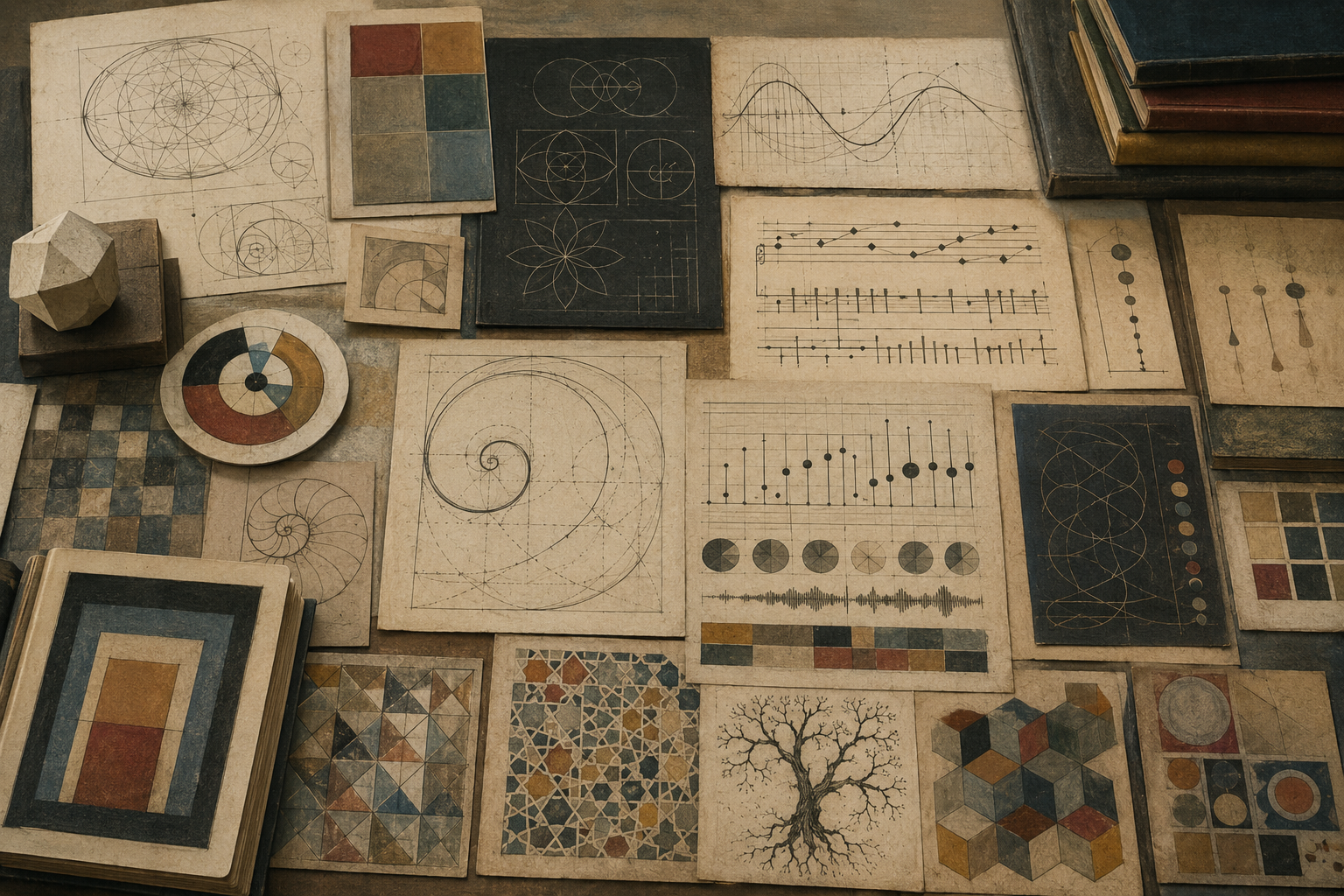
Mathematics, Art, Music, and Pattern examines the deep relationships among proportion, symmetry, rhythm, geometry, tuning, repetition, variation, structure, and aesthetic meaning. This article map explores how mathematical forms appear in visual art, architecture, music, design, nature, computation, and human perception.
Mathematics is not only a tool for calculation. It is also a language of pattern, relation, transformation, proportion, order, and surprise. Art and music are not only expressive practices. They often depend on structure, interval, recurrence, contrast, scale, sequence, and formal tension. Between mathematics and the arts lies a shared concern with how forms hold together and why certain patterns feel meaningful.
This article map sits within the broader Meaning category. Its focus is interpretive and generative: how mathematical pattern participates in aesthetic experience, how artistic and musical forms reveal mathematical structure, and how computational tools can support responsible exploration without reducing art or music to formulas alone.
Mathematics, Art, Music, and Pattern provides a bridge between formal structure and aesthetic experience. It asks why certain proportions feel balanced, why symmetry can appear beautiful or static, why rhythm organizes time, why repetition invites memory, why variation creates interest, and why mathematical structures appear so frequently in visual and musical forms.
This map does not claim that mathematics explains all beauty. Art and music cannot be reduced to equations, ratios, or algorithms. Yet mathematical thinking helps clarify many of the relationships that make aesthetic form intelligible: scale, sequence, interval, recurrence, contrast, transformation, proportion, density, periodicity, continuity, and complexity.
The articles in this map move from foundations of pattern and aesthetic order into geometry, visual form, musical structure, algorithmic creation, cognition, complexity, interpretation, ethics, and responsible tool use. Together, they provide a research pathway for understanding how mathematical form participates in art, music, design, perception, and meaning.
GitHub Repository
This article map is supported by companion research scaffolding for pattern analysis, geometric studies, musical interval models, rhythm and cycle experiments, generative art workflows, design studies, synthetic teaching datasets, visual archives, and reproducible computational exploration.
Complete Code Repository
The Mathematics, Art, Music, and Pattern companion repository includes article-level folders, pattern datasets, geometry examples, rhythm and tuning studies, generative art scripts, visual-composition notes, music-structure models, documentation, Python workflows, R summaries, SQL catalogs, notebooks, Canvas cards, and reproducible studio-lab scaffolding for mathematical and aesthetic exploration.
Mathematics, Art, Music, and Pattern as a Field of Meaning
Mathematics, art, music, and pattern belong together because they all ask how forms relate. A visual composition depends on proportion, balance, contrast, rhythm, scale, and structure. A musical work depends on interval, recurrence, duration, tension, resolution, and transformation. A mathematical pattern depends on relation, rule, symmetry, sequence, mapping, or invariant structure. These domains are not identical, but they share a concern with ordered difference.
Pattern is one of the ways human beings recognize meaning. A repeated figure becomes memorable. A variation becomes intelligible because it differs from something already known. A rhythm creates expectation. A proportion creates relation. A symmetry creates balance or tension. A transformation allows one form to become another without losing identity. These are not only mathematical ideas. They are aesthetic experiences.
This field therefore studies the intersection between formal structure and lived perception. It asks why geometry can feel elegant, why musical ratios can sound consonant or tense, why visual rhythms organize space, why spirals and fractals feel organic, why complexity can be pleasurable, and why some patterns become culturally, spiritually, or emotionally significant.
Mathematics, Art, Music, and Pattern treats mathematical form as a resource for interpretation rather than a replacement for interpretation. Mathematics helps describe relationships, but art and music remain historical, cultural, embodied, expressive, and meaningful in ways that exceed formal structure alone.
Why Pattern Belongs Under Meaning
Pattern belongs under Meaning because human beings do not simply perceive isolated objects. They perceive relations, rhythms, contrasts, recurrences, and transformations. Meaning often emerges when elements are not merely present, but organized. A color field becomes a composition. A sound becomes a melody. A sequence becomes a rhythm. A repeated motif becomes a symbol. A proportional relationship becomes a structure of expectation.
Pattern also helps explain why form can feel meaningful before it is translated into language. A curve, chord, grid, cadence, spiral, tessellation, or rhythmic cycle may be experienced as ordered, tense, playful, solemn, sacred, chaotic, or resolved. These meanings do not depend entirely on words. They arise through embodied perception, cultural learning, memory, and attention to form.
Mathematics gives pattern a precise language. It can describe symmetry groups, ratios, intervals, recurrences, transformations, waves, proportions, tilings, networks, scaling laws, and periodic structures. But Meaning asks a different question: what do these patterns do in human experience? How do they organize perception, emotion, memory, ritual, attention, and interpretation?
This article map belongs in the Meaning category because it shows how formal structure becomes aesthetic significance. It connects mathematical reasoning to artistic perception, musical time, cultural pattern, computational creation, and philosophical reflection.
What This Article Map Studies
This article map studies the ways mathematical ideas appear in art, music, architecture, design, nature, cognition, and computation. It includes proportion, ratio, symmetry, asymmetry, repetition, variation, geometry, perspective, projection, tessellation, curves, spirals, fractals, topology, musical intervals, tuning systems, rhythm, cycles, Fourier thinking, algorithmic art, generative design, cellular automata, randomness, complexity, and mathematical beauty.
At the visual level, it examines geometry, proportion, perspective, tiling, scale, curvature, symmetry, transformation, and emergent form. At the musical level, it studies intervals, ratios, tuning systems, rhythm, meter, cycles, polyrhythm, timbre, Fourier decomposition, and musical transformation. At the computational level, it studies generative art, procedural music, algorithmic pattern, cellular automata, chance operations, controlled variation, and code as a studio tool.
At the interpretive level, it studies why patterns feel meaningful. This includes Gestalt perception, prediction and surprise, simplicity and complexity, order and chaos, mathematical beauty, and the risk of confusing formal explanation with aesthetic understanding. At the ethical level, it studies authorship, AI-generated art, cultural pattern, appropriation, over-mathematization, and the responsibilities of computational creation.
The goal is to create a research pathway that respects both formal rigor and aesthetic depth. Mathematics can illuminate art and music, but the illumination must remain interpretive, historically aware, and culturally responsible.
Major Themes in Mathematics, Art, Music, and Pattern
One major theme is proportion. Proportion links parts to wholes. It appears in architecture, painting, design, sculpture, typography, music, and natural form. Proportion can produce harmony, tension, monumentality, intimacy, rhythm, or imbalance depending on context.
A second theme is symmetry and transformation. Symmetry creates order, but too much symmetry can feel static. Asymmetry can create movement, emphasis, and expressive tension. Transformations allow forms to shift, rotate, scale, repeat, invert, or develop while retaining recognizable structure.
A third theme is rhythm. Rhythm is pattern in time, but it also appears visually through spacing, recurrence, alternation, and repetition. In music, rhythm organizes attention and expectation. In visual art and design, rhythm organizes movement across a surface.
A fourth theme is geometry. Geometry shapes how space is imagined, constructed, represented, and interpreted. Perspective, projection, tiling, curves, spirals, grids, and topology all show how mathematical structures can organize visual worlds.
A fifth theme is complexity. Patterns can be simple, complex, random, ordered, chaotic, emergent, or layered. Aesthetic pleasure often depends on the balance between predictability and surprise, clarity and depth, order and variation.
A sixth theme is generation. Algorithms, rules, procedures, constraints, and computational systems can produce images, music, patterns, and forms. But generative methods raise interpretive and ethical questions about authorship, intention, craft, culture, originality, and the limits of automation.
Mathematics, Art, Music, and Pattern Article Map
The map below organizes the Mathematics, Art, Music, and Pattern series into six parts, moving from foundations of pattern and aesthetic order into geometry, music, algorithmic form, cognition, complexity, ethics, and responsible interpretation.
Part I — Foundations of Pattern and Aesthetic Order
- Pattern as a Bridge Between Mathematics and Art (planned) — A foundational article on how pattern links mathematical relation, artistic form, musical structure, and aesthetic meaning.
- Mathematical Thinking in Aesthetic Form (planned) — An article on how abstraction, relation, transformation, and structure appear in art, music, and design.
- Proportion, Ratio, and Aesthetic Order (planned) — A study of how ratios and proportional systems organize visual and musical experience.
- Symmetry, Asymmetry, and Visual Meaning (planned) — An article on balance, reflection, rotation, variation, visual tension, and the aesthetic force of ordered difference.
- Repetition, Variation, and Structure (planned) — A focused article on motif, recurrence, difference, development, memory, rhythm, and formal coherence.
- Why Patterns Feel Meaningful (planned) — An article on perception, expectation, recognition, embodiment, culture, and the emotional force of structured relation.
Part II — Geometry and Visual Form
- Geometry in Art and Architecture (planned) — An article on how geometric structures shape buildings, paintings, ornament, design systems, and sacred spaces.
- Perspective, Projection, and the Mathematics of Seeing (planned) — A study of visual representation, projection, depth, viewpoint, pictorial space, and mathematical perspective.
- Tessellation, Tiling, and Repetition (planned) — An article on repeating forms, plane-filling patterns, modular order, ornament, and visual rhythm.
- Curves, Spirals, and Organic Form (planned) — A focused article on curved structures, spirals, growth patterns, motion, and the aesthetics of organic geometry.
- Fractals, Scaling, and Natural Pattern (planned) — A study of self-similarity, scaling, branching, natural form, visual complexity, and mathematical pattern in nature.
- Topology, Continuity, and Visual Transformation (planned) — An article on continuity, deformation, connectedness, surfaces, knots, and transformation as aesthetic ideas.
Part III — Mathematics and Music
- Intervals, Ratios, and Musical Sound (planned) — An article on musical intervals, frequency ratios, consonance, dissonance, and the mathematical structure of pitch relations.
- Tuning Systems and Temperament (planned) — A study of just intonation, equal temperament, tuning compromises, cultural systems, and the mathematical organization of pitch.
- Rhythm, Meter, and Mathematical Time (planned) — An article on duration, pulse, meter, periodicity, subdivision, and the temporal mathematics of music.
- Polyrhythm, Cycles, and Layered Pattern (planned) — A focused article on overlapping cycles, rhythmic complexity, cross-rhythm, repetition, and embodied musical time.
- Symmetry and Transformation in Music (planned) — An article on inversion, retrograde, transposition, variation, canon, sequence, and musical transformation.
- Fourier Thinking, Timbre, and Sound Structure (planned) — A study of waves, overtones, spectral structure, sound decomposition, timbre, and the mathematics of musical color.
Part IV — Algorithmic and Generative Form
- Algorithmic Art and Rule-Based Creation (planned) — An article on using explicit rules, procedures, constraints, and formal systems to generate visual art.
- Generative Design and Computational Pattern (planned) — A study of computational systems that produce patterns, layouts, forms, variations, and design possibilities.
- Cellular Automata and Visual Complexity (planned) — An article on simple rules, emergent behavior, grid-based systems, and the aesthetics of computational complexity.
- Randomness, Chance, and Controlled Variation (planned) — A focused article on aleatory methods, stochastic form, controlled chance, and the artistic use of uncertainty.
- Procedural Music and Generative Composition (planned) — An article on algorithmic composition, rule-based sound, procedural variation, and computational musical form.
- Code as a Studio Tool for Pattern Exploration (planned) — A practical article on using code to explore pattern, geometry, rhythm, color, form, and variation without replacing artistic judgment.
Part V — Cognition, Complexity, and Interpretation
- Gestalt Principles and Mathematical Form (planned) — An article on grouping, closure, proximity, similarity, figure-ground relations, and perceptual organization.
- Pattern Recognition and Aesthetic Perception (planned) — A study of how human beings identify structure, relation, recurrence, and difference in visual and musical forms.
- Prediction, Surprise, and Aesthetic Pleasure (planned) — An article on expectation, violation, resolution, novelty, and the pleasures of structured uncertainty.
- Complexity, Simplicity, and Aesthetic Balance (planned) — A focused article on the tension between clarity and richness, minimalism and density, order and variety.
- Order, Chaos, and Emergent Form (planned) — An article on complex systems, generative processes, nonlinear patterns, emergence, and aesthetic interpretation.
- Why Mathematical Beauty Is Not Just Formal (planned) — A philosophical article on elegance, insight, surprise, intelligibility, meaning, and the limits of purely formal explanation.
Part VI — Ethics, Tools, and Limits
- Can Mathematics Explain Beauty? (planned) — A critical article on what mathematical analysis can and cannot explain about aesthetic value.
- The Risk of Over-Mathematizing Art (planned) — An article on reductionism, false precision, cultural erasure, and the danger of treating art as pattern alone.
- Computational Tools for Pattern Analysis (planned) — A practical article on responsible uses of computational tools for studying visual, musical, and generative patterns.
- Mathematical Pattern Across Cultures (planned) — A study of pattern traditions, ornament, architecture, music, craft, ritual, and cultural context.
- AI, Generative Art, and Authorship (planned) — A critical article on AI-generated images and music, originality, credit, training data, style, authorship, and human agency.
- Mathematics, Art, Music, and Pattern: A Capstone (planned) — A capstone article on formal structure, aesthetic meaning, computation, culture, interpretation, and responsible creation.
Python Workflow: Generative Patterns, Geometry, and Musical Structure
A useful Python workflow for this article map is a generative pattern and structure workflow. The workflow can begin with simple rules for grids, spirals, tessellations, symmetry transformations, rhythmic cycles, or pitch ratios. Python can then generate visual studies, structured datasets, pattern inventories, SVG-style diagrams, Markdown summaries, and reproducible outputs for teaching and article drafting.
This workflow belongs naturally with articles on geometry, tessellation, fractals, algorithmic art, procedural music, cellular automata, and computational pattern. For example, a Python script can generate a grid of rotated motifs, simulate a cellular automaton, compare rhythmic cycles, calculate interval ratios, or export a table of transformations used in a visual composition.
The workflow should not suggest that code replaces artistic practice. Its role is exploratory. Code can help reveal formal possibilities, compare structures, generate variations, document assumptions, and support reproducible studio experiments. Interpretation still belongs to the human researcher, artist, musician, designer, or reader.
R Workflow: Pattern Comparison, Rhythm Summaries, and Aesthetic Structures
A useful R workflow for this article map is a pattern-comparison and aesthetic-structure workflow. A structured teaching dataset can include article titles, pattern types, visual domains, musical domains, mathematical concepts, cultural contexts, computational methods, and interpretive cautions. R can summarize recurring themes, compare pattern categories, and generate tables for research planning.
This workflow belongs naturally with articles on proportion, symmetry, rhythm, musical intervals, complexity, perception, and mathematical beauty. For example, R can help summarize which articles focus on geometry, which focus on music, which focus on computation, which focus on cognition, and which focus on ethics. It can also support comparative reading notes across visual, musical, and mathematical traditions.
As with the Python workflow, the goal is not to reduce aesthetic meaning to a dataset. The goal is to make research organization more transparent. Pattern analysis becomes more useful when its categories, assumptions, examples, and limitations are visible.
Ethics, Interpretation, and the Risk of Over-Mathematizing Art
Mathematics can illuminate art and music, but it can also distort them when used carelessly. A painting is not meaningful only because it contains a ratio. A musical tradition is not valuable only because it can be translated into frequency relationships. A cultural pattern is not fully understood because it can be classified, tiled, modeled, or generated. Formal analysis must remain accountable to context, history, material, culture, practice, and lived experience.
The risk of over-mathematizing art is the risk of treating structure as the whole of meaning. Mathematical description can make patterns visible, but it may miss ritual context, symbolic association, craft knowledge, embodied technique, spiritual meaning, political history, cultural authority, or emotional resonance. A serious approach must ask not only what pattern is present, but what the pattern is doing in a particular world.
Computation adds another ethical layer. Generative systems can imitate styles, produce endless variations, and abstract cultural forms into reusable datasets. That power requires responsibility. Questions of authorship, consent, attribution, training data, cultural borrowing, and interpretive care matter deeply when mathematical and computational tools enter artistic and musical domains.
The ethical goal is not to avoid mathematics. The goal is to use mathematical and computational tools with humility. Pattern can be studied rigorously without flattening art, music, culture, or beauty into mechanism alone.
Mathematics, Art, Music, and Pattern in a Wider Intellectual Context
Mathematics, Art, Music, and Pattern belongs within a wider knowledge architecture because pattern links perception, reasoning, aesthetics, culture, and creation. It sits under Meaning because mathematical form becomes significant only when it enters human attention, practice, interpretation, and experience.
This map also connects to aesthetics and the philosophy of art through beauty, judgment, form, and interpretation. It connects to music theory through intervals, rhythm, tuning, form, timbre, and performance. It connects to design through grids, proportion, color systems, typography, visual rhythm, and generative layout. It connects to scientific computing and algorithms through code, simulation, procedural generation, cellular automata, and AI-generated form.
By giving mathematics, art, music, and pattern their own article map, the site treats formal structure as a serious part of human meaning. Pattern is not merely decorative. It is one of the ways human beings perceive relation, organize time, imagine space, recognize order, experience surprise, and create worlds of form.
Related Reading
- Meaning
- Beauty, Aesthetics, and Meaning
- Aesthetics and the Philosophy of Art
- Color Theory, Typography, and Design
- Music Theory, Form, and Meaning
- Symbolism, Style, and Cultural Meaning
- Creative Form, Composition, and Interpretation
- Algorithms and Computational Reasoning
Further Reading
- Arnheim, R. (1974). Art and Visual Perception: A Psychology of the Creative Eye. Berkeley: University of California Press.
- Barrow, J.D. (1995). The Artful Universe: The Cosmic Source of Human Creativity. Oxford: Oxford University Press.
- Bell, J. (1999). The Art of Mathematics: Coffee Time in Memphis. Cambridge: Cambridge University Press.
- Ghyka, M. (1977). The Geometry of Art and Life. New York: Dover Publications.
- Godwin, J. (1992). Harmonies of Heaven and Earth: The Spiritual Dimension of Music from Antiquity to the Avant-Garde. Rochester, VT: Inner Traditions.
- Hofstadter, D.R. (1979). Gödel, Escher, Bach: An Eternal Golden Braid. New York: Basic Books.
- Livio, M. (2002). The Golden Ratio: The Story of Phi, the World’s Most Astonishing Number. New York: Broadway Books.
- Mandelbrot, B.B. (1982). The Fractal Geometry of Nature. New York: W.H. Freeman.
- Maor, E. (2018). Music by the Numbers: From Pythagoras to Schoenberg. Princeton: Princeton University Press.
- McClain, E.G. (1976). The Myth of Invariance: The Origin of the Gods, Mathematics and Music from the Rg Veda to Plato. York Beach, ME: Nicolas-Hays.
- Stewart, I. (2001). What Shape Is a Snowflake? Magical Numbers in Nature. London: Weidenfeld & Nicolson.
- Weyl, H. (1952). Symmetry. Princeton: Princeton University Press.
References
- Arnheim, R. (1974). Art and Visual Perception: A Psychology of the Creative Eye. Berkeley: University of California Press.
- Barrow, J.D. (1995). The Artful Universe: The Cosmic Source of Human Creativity. Oxford: Oxford University Press.
- Bell, J. (1999). The Art of Mathematics: Coffee Time in Memphis. Cambridge: Cambridge University Press.
- Coxeter, H.S.M. (1969). Introduction to Geometry, 2nd edn. New York: Wiley.
- Ghyka, M. (1977). The Geometry of Art and Life. New York: Dover Publications.
- Godwin, J. (1992). Harmonies of Heaven and Earth: The Spiritual Dimension of Music from Antiquity to the Avant-Garde. Rochester, VT: Inner Traditions.
- Hofstadter, D.R. (1979). Gödel, Escher, Bach: An Eternal Golden Braid. New York: Basic Books.
- Iversen, M. (1993). Alois Riegl: Art History and Theory. Cambridge, MA: MIT Press.
- Kappraff, J. (2001). Connections: The Geometric Bridge Between Art and Science, 2nd edn. Singapore: World Scientific.
- Livio, M. (2002). The Golden Ratio: The Story of Phi, the World’s Most Astonishing Number. New York: Broadway Books.
- Mandelbrot, B.B. (1982). The Fractal Geometry of Nature. New York: W.H. Freeman.
- Maor, E. (2018). Music by the Numbers: From Pythagoras to Schoenberg. Princeton: Princeton University Press.
- McClain, E.G. (1976). The Myth of Invariance: The Origin of the Gods, Mathematics and Music from the Rg Veda to Plato. York Beach, ME: Nicolas-Hays.
- Penrose, R. (1974). ‘The role of aesthetics in pure and applied mathematical research’, Bulletin of the Institute of Mathematics and its Applications, 10, pp. 266–271.
- Stewart, I. (2001). What Shape Is a Snowflake? Magical Numbers in Nature. London: Weidenfeld & Nicolson.
- Tymoczko, D. (2011). A Geometry of Music: Harmony and Counterpoint in the Extended Common Practice. Oxford: Oxford University Press.
- Weyl, H. (1952). Symmetry. Princeton: Princeton University Press.
- Williams, K. (1998). Nexus: Architecture and Mathematics. Fucecchio: Edizioni dell’Erba.