
Last Updated June 6, 2026
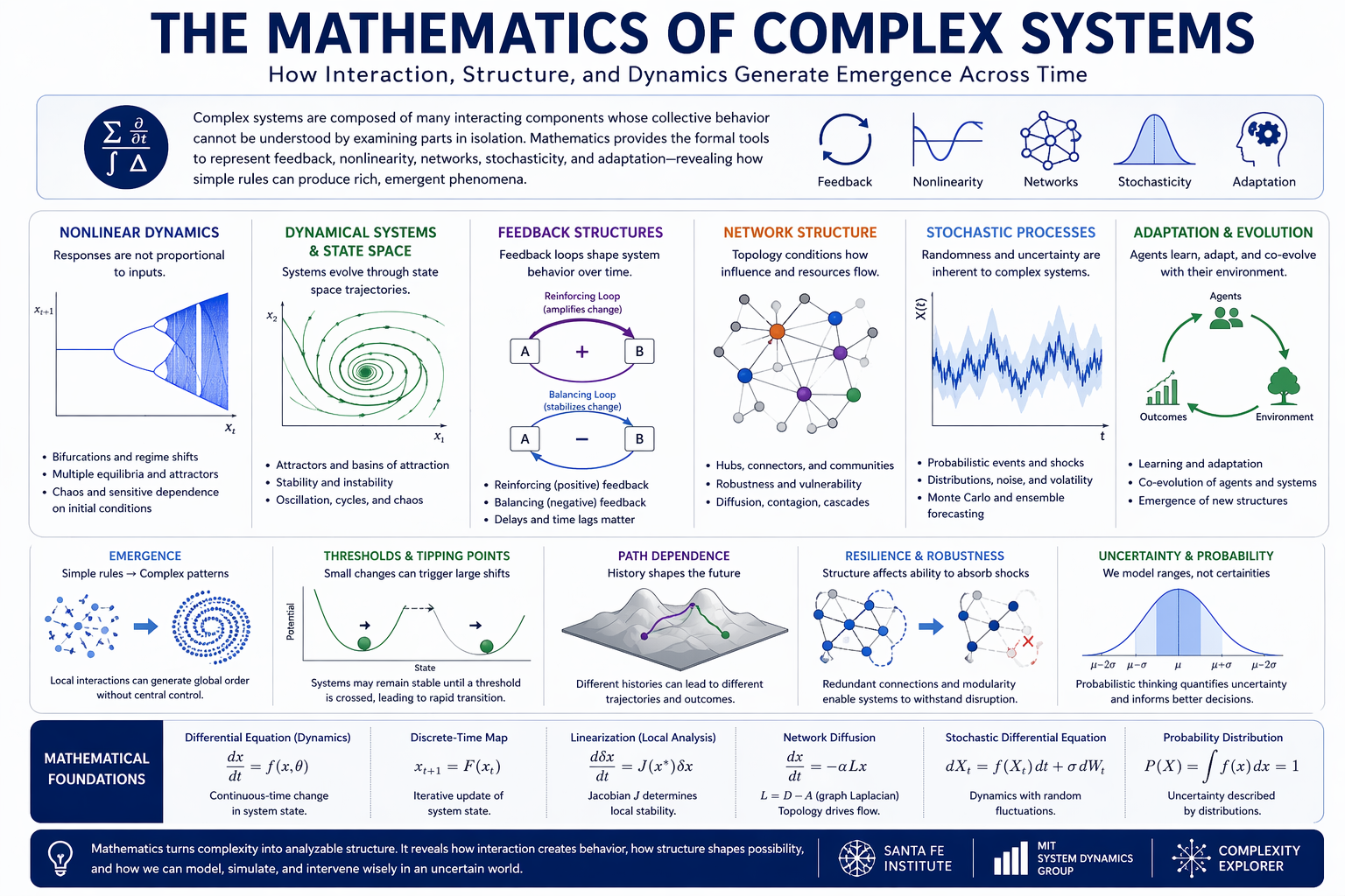
The mathematics of complex systems provides the formal analytical language through which interacting components generate dynamic, emergent behavior across natural, technological, economic, ecological, organizational, and social systems. Systems modeling depends on mathematical tools drawn from nonlinear dynamics, dynamical systems theory, graph theory, stochastic processes, information theory, statistical mechanics, optimization, computational simulation, and uncertainty analysis. These tools make it possible to represent feedback, accumulation, adaptation, thresholds, contagion, resilience, path dependence, and structural interdependence with more discipline than intuition alone can provide.
Complex systems often behave in ways that simple linear reasoning cannot explain. Small changes may produce large consequences. Delays may generate oscillation. Local interaction may create global order. Network structure may determine whether shocks remain contained or cascade across a system. Random disturbance may interact with deterministic structure. Adaptive agents may change the conditions to which they respond. Mathematical representation helps make these processes explicit, testable, comparable, and interpretable.
The mathematics of complex systems is not one single method. It is a family of formal languages for representing how structure generates behavior over time. Differential equations, difference equations, matrices, graphs, probability distributions, transition rules, simulation algorithms, information measures, and stability criteria each illuminate different aspects of complex behavior. The art of systems modeling lies in choosing mathematical representations that are appropriate to the system, the evidence, the decision context, and the limits of interpretation.

This article explains the mathematics of complex systems as a bridge between conceptual systems thinking and formal systems modeling. It covers nonlinear dynamics, dynamical systems, state space, feedback, stability, emergence, network mathematics, stochastic processes, adaptation, entropy, computational complexity, scaling, spatial systems, mathematical interpretation, sustainability and policy implications, professional workflows, R and Python examples, responsible use, common pitfalls, and authoritative references.
Why Complex Systems Require Mathematical Representation
Complex systems require mathematical representation because their behavior often depends on relationships that are difficult to reason about verbally. Feedback, delay, accumulation, adaptation, nonlinear response, stochastic disturbance, network structure, and cross-scale interaction can produce outcomes that are counterintuitive even when the individual pieces seem understandable.
Mathematics provides a disciplined way to represent these relationships. It makes assumptions explicit. It identifies variables and parameters. It defines state, change, interaction, probability, constraint, and performance. It allows analysts to test whether a proposed explanation actually produces the behavior it claims to explain. It also makes it possible to compare models across domains that otherwise appear unrelated.
For example, predator-prey cycles, traffic congestion, financial contagion, epidemic spread, social imitation, power-grid instability, institutional lock-in, and climate feedback may involve different subject matter. Yet each can involve formal patterns such as coupled dynamics, threshold behavior, network diffusion, stochastic transition, or nonlinear amplification. Mathematics provides the shared language for recognizing these patterns.
| Complex-system feature | Why intuition struggles | Mathematical representation |
|---|---|---|
| Feedback | Effects loop back into causes over time. | Recursive equations, differential equations, causal loop structure. |
| Delay | Actions produce effects later, often after conditions have changed. | Lagged variables, delay differential equations, discrete event logic. |
| Nonlinearity | Effects are not proportional to causes. | Nonlinear functions, bifurcation analysis, threshold models. |
| Emergence | System-level order arises from local interaction. | Agent rules, network interaction, statistical mechanics, simulation. |
| Uncertainty | Outcomes depend on incomplete knowledge and random disturbance. | Probability distributions, stochastic processes, ensembles. |
| Network dependence | Relationships shape behavior as much as individual attributes. | Graphs, adjacency matrices, centrality, Laplacians, diffusion models. |
| Adaptation | Agents learn, adjust, imitate, avoid, or redesign behavior. | Evolutionary dynamics, game theory, reinforcement rules, adaptive agents. |
This is why mathematics sits near the intellectual core of Why Complex Systems Require Models and Core Principles of Systems Modeling. It is the formal grammar through which systemic behavior becomes analyzable.
What Counts as the Mathematics of Complex Systems?
The mathematics of complex systems includes any formal language that helps represent how interacting parts generate collective behavior. It is broader than equations alone. It includes equations, graphs, matrices, probability models, transition rules, optimization criteria, simulation algorithms, stability conditions, information measures, and computational experiments.
Different mathematical tools answer different questions. A differential equation may describe how a stock changes continuously through time. A graph may describe who depends on whom. A stochastic process may describe uncertain transitions. An agent-based rule set may describe decentralized adaptation. A matrix may represent flows, dependencies, or state transitions. A simulation may reveal behavior that cannot be solved cleanly in closed form.
The point is not to make systems modeling look mathematically elaborate. The point is to choose the simplest formal representation that is strong enough to represent the system behavior under study.
| Formal object | What it represents | Systems modeling use |
|---|---|---|
| State variable | A measurable condition of the system. | Population, inventory, capacity, trust, temperature, debt, infection count. |
| Parameter | A value governing system behavior. | Growth rate, recovery rate, failure probability, diffusion strength. |
| Function | A rule connecting inputs to outputs. | Response curves, production functions, damage functions, adoption rules. |
| Matrix | Structured relationships among many variables. | Network adjacency, transition probability, input-output flows. |
| Graph | Nodes and relationships. | Infrastructure, contagion, influence, supply chains, ecological food webs. |
| Distribution | Probabilistic uncertainty or variation. | Demand, failure times, shocks, service times, behavioral response. |
| Algorithm | A computational procedure. | Simulation, optimization, search, calibration, agent interaction. |
Mathematical representation should always be tied to interpretive purpose. A model that is mathematically sophisticated but poorly matched to the system can mislead more than a simpler model whose assumptions are clear.
Major Mathematical Frameworks
Complex systems mathematics draws from several overlapping traditions. Each framework highlights a different aspect of system behavior: change over time, relational structure, uncertainty, adaptation, information, scaling, or computation.
Dynamical Systems
Dynamical systems theory studies how system states evolve through time. It provides tools for analyzing equilibria, attractors, stability, oscillation, chaos, bifurcation, and transitions between behavior regimes.
Nonlinear Dynamics
Nonlinear dynamics examines systems where outputs are not proportional to inputs. It is central to thresholds, tipping points, saturation, runaway growth, feedback amplification, and sensitive dependence on initial conditions.
Graph Theory and Network Science
Graph theory represents systems as nodes and edges. It helps analyze centrality, clustering, modularity, diffusion, contagion, dependency, robustness, and cascading failure.
Stochastic Processes
Stochastic processes represent probabilistic change through time. They are used for random shocks, noisy observations, uncertain transitions, reliability, epidemics, queues, and risk analysis.
Statistical Mechanics
Statistical mechanics connects micro-level interaction with macro-level patterns. It is useful for studying emergence, phase transitions, collective behavior, scaling, and many-agent systems.
Information Theory
Information theory provides tools for measuring uncertainty, entropy, redundancy, signal structure, diversity, predictability, and informational organization in dynamic systems.
Optimization and Control
Optimization and control theory help evaluate interventions, constraints, stability, tradeoffs, adaptive policies, feedback control, and decision rules under uncertainty.
Computational Simulation
Simulation allows analysts to explore systems that cannot be solved analytically. It supports scenario exploration, agent interaction, stochastic ensembles, stress testing, and model comparison.
| Framework | Primary question | Typical systems modeling application |
|---|---|---|
| Dynamical systems | How does the system evolve through time? | Population dynamics, climate feedback, economic cycles, resource depletion. |
| Network science | How does structure shape flow, influence, or failure? | Infrastructure, contagion, supply chains, communication, ecosystems. |
| Stochastic processes | How does uncertainty affect trajectories? | Reliability, epidemics, demand variation, service systems, risk. |
| Statistical mechanics | How do many local interactions create macro patterns? | Emergence, phase transitions, collective behavior, scaling. |
| Information theory | How much uncertainty, structure, or signal exists? | Entropy, diversity, predictability, system organization. |
| Optimization | Which action performs best under constraints? | Resource allocation, policy design, robust decisions, control. |
| Simulation | What behavior emerges under specified rules? | Agent-based models, scenario ensembles, stress tests, hybrid models. |
The strength of complex systems mathematics lies in combining these frameworks carefully. A public-health model may use differential equations, stochastic processes, networks, and optimization. An infrastructure model may combine graph theory, reliability analysis, discrete events, and stress testing. A climate policy model may combine coupled dynamics, uncertainty ensembles, and robust decision analysis.
Nonlinear Dynamics and System Behavior
Many complex systems are governed by nonlinear dynamics, meaning that system responses are not proportional to changes in inputs. In a linear system, doubling an input tends to double the output. In a nonlinear system, doubling an input may produce almost no change, a moderate change, a runaway change, or a qualitative transition into a different regime.
Nonlinearity matters because it is one of the main reasons complex systems surprise us. A system may absorb stress for a long time and then suddenly fail. A small intervention may have little effect until it reaches a threshold. A feedback loop may amplify change gradually, then explosively. A stable pattern may become unstable when a parameter crosses a critical value.
Nonlinear dynamics are often represented through differential equations, difference equations, recurrence relations, response functions, saturation curves, and threshold rules. These forms can generate oscillation, path dependence, bifurcation, tipping behavior, chaotic trajectories, or multiple equilibria.
| Nonlinear behavior | Meaning | Example |
|---|---|---|
| Saturation | Growth slows as a limit is approached. | Resource-limited population, market adoption, infrastructure capacity. |
| Threshold | Behavior changes after a critical point. | Grid overload, ecosystem collapse, disease outbreak, queue failure. |
| Bifurcation | A small parameter change alters qualitative behavior. | Stable equilibrium becomes oscillatory or unstable. |
| Chaos | Deterministic rules produce long-run unpredictability. | Sensitive dependence on initial conditions. |
| Hysteresis | Return path differs from departure path. | Degraded ecosystems, institutional lock-in, material fatigue. |
| Positive feedback | Change reinforces itself. | Runaway growth, cumulative advantage, speculative bubbles. |
Nonlinear dynamics connect directly to System Dynamics Modeling, Critical Transitions and Tipping Points in Complex Systems, and Stress Testing and Robustness Analysis.
Dynamical Systems and State-Space Analysis
Dynamical systems theory provides one of the most general mathematical frameworks for analyzing how systems evolve over time. In this approach, the state of a system is represented as a vector whose components describe the condition of the system at a given moment. The set of all possible states forms a multidimensional space known as the state space.
A trajectory through state space describes how the system changes according to its governing rules. Mathematical analysis of these trajectories allows researchers to identify attractors, basins of attraction, stable equilibria, unstable equilibria, oscillatory regimes, transient dynamics, and transitions between qualitatively different behavior modes.
State-space analysis is useful because it shifts attention from isolated events to the geometry of system behavior. A system is not only a sequence of outcomes. It is a landscape of possible states, pathways, constraints, and regions of attraction. This perspective is especially important for resilience, tipping points, path dependence, and adaptive systems.
| State-space concept | Meaning | Systems modeling relevance |
|---|---|---|
| State vector | A collection of variables describing the system condition. | Population, resources, capacity, emissions, trust, demand, debt. |
| Trajectory | The path a system follows through state space. | Growth path, collapse path, recovery path, transition pathway. |
| Equilibrium | A state where the system does not change under current rules. | Stable population, balanced flow, steady service level. |
| Attractor | A region or pattern toward which trajectories tend. | Stable regime, cycle, lock-in, persistent behavior pattern. |
| Basin of attraction | The set of initial conditions leading to an attractor. | Resilience, regime stability, transition risk. |
| Transient behavior | Temporary dynamics before long-run pattern emerges. | Policy transition, recovery, adjustment, short-term instability. |
Some systems display chaotic dynamics, in which trajectories diverge rapidly despite almost identical initial conditions. This limits long-run prediction even when the system is deterministic. Chaos therefore shows that uncertainty in complex systems is not always caused by randomness; it can emerge from deterministic dynamics that amplify small differences over time.
Feedback Structures and System Stability
Feedback relationships are fundamental to the mathematics of complex systems. Reinforcing feedback amplifies change and may generate exponential growth, cumulative advantage, runaway instability, or collapse. Balancing feedback counteracts deviation and contributes to stability, regulation, or homeostasis.
Mathematically, feedback is often represented through coupled equations linking variables recursively through time. The stability of the resulting system depends on both the strength and configuration of those couplings. Small changes in feedback structure can produce major differences in behavior, including convergence, oscillation, overshoot, collapse, or divergence.
Feedback is central to engineering control systems, ecological regulation, economic cycles, organizational learning, climate dynamics, and public policy. In systems modeling, feedback is one of the main mechanisms through which structure generates behavior.
| Feedback concept | Mathematical representation | System behavior |
|---|---|---|
| Reinforcing feedback | Positive feedback coefficient or self-amplifying recurrence. | Growth, escalation, lock-in, cumulative advantage. |
| Balancing feedback | Negative feedback coefficient or corrective control rule. | Stabilization, regulation, goal-seeking behavior. |
| Delayed feedback | Lagged variable or delayed response term. | Oscillation, overshoot, policy resistance. |
| Nonlinear feedback | Feedback strength changes with state. | Thresholds, saturation, instability, regime shifts. |
| Coupled feedback | Multiple feedback loops interact. | Complex dynamics, competing effects, emergent behavior. |
| Control feedback | Policy rule adjusts action based on deviation from target. | Correction, stabilization, adaptive control. |
This makes the mathematics of feedback indispensable for Modeling Feedback Loops, Delay, Oscillation, and Policy Resistance, and Leverage Points in Complex Systems.
Emergence and Collective Dynamics
Emergence occurs when large-scale patterns arise from local interactions among components without requiring centralized control. Mathematics provides several ways to analyze this process. Agent-based models formalize decentralized interaction through rules. Network mathematics captures how topology conditions contact and influence. Statistical mechanics explains how macro-level regularities can arise from many interacting micro-units. Mean-field approximations summarize the aggregate effect of many individuals.
Emergent order can appear in markets, traffic, ecosystems, organizations, social norms, flocking behavior, institutional routines, technological adoption, and collective risk perception. In each case, system behavior cannot be understood by analyzing isolated components alone. The interaction structure matters.
Markets
Prices, bubbles, crashes, and liquidity patterns can emerge from decentralized trading, expectations, leverage, feedback, and network exposure.
Traffic
Congestion waves can emerge from local braking, lane changes, reaction times, capacity limits, and route choice.
Ecosystems
Food webs, population cycles, biodiversity patterns, and regime shifts emerge from many interacting species and environmental conditions.
Organizations
Culture, bottlenecks, coordination failures, learning patterns, and institutional inertia emerge from routines, incentives, roles, and communication paths.
Technology Adoption
Diffusion patterns emerge from peer influence, thresholds, network structure, perceived value, cost, and institutional support.
Public Behavior
Compliance, panic, trust, protest, migration, and norm change can emerge from local information, identity, risk perception, and social influence.
Emergence illustrates why complex systems cannot always be understood by decomposing them into parts and summing their properties. This is precisely why Agent-Based Modeling and Network Models are mathematically and conceptually central to contemporary systems modeling.
Network Mathematics and System Structure
Many complex systems can be represented as networks: collections of nodes linked by edges. Network theory and graph theory provide the mathematics for analyzing how system topology influences diffusion, coordination, robustness, vulnerability, and cascading failure.
Nodes may represent people, organizations, infrastructure assets, species, firms, documents, machines, neighborhoods, or institutions. Edges may represent contact, dependency, flow, influence, trade, communication, transmission, similarity, or control. Once represented as a network, the system can be analyzed using graph measures that reveal structural position and relational vulnerability.
| Network measure | Meaning | Systems modeling use |
|---|---|---|
| Degree | Number of connections a node has. | Exposure, influence, dependency, hub identification. |
| Betweenness centrality | How often a node lies on shortest paths. | Bottlenecks, brokers, bridge nodes, chokepoints. |
| Closeness centrality | Average distance from one node to others. | Access, reachability, diffusion speed. |
| Eigenvector centrality | Influence based on connection to influential nodes. | Authority, systemic importance, prestige, exposure. |
| Clustering | Degree to which neighbors connect to each other. | Local cohesion, redundancy, contagion pockets. |
| Modularity | Strength of community structure. | Subsystem detection, fragmentation, resilience planning. |
| Path length | Distance between nodes. | Diffusion, accessibility, failure propagation. |
Network mathematics has become essential for analyzing communication systems, social influence, transportation, power grids, supply chains, epidemiological transmission, ecological webs, financial contagion, and cyber-physical infrastructure. It demonstrates that system behavior is shaped not only by the attributes of parts, but by the architecture of relationships linking them.
Stochastic Processes and Uncertainty
Real-world systems frequently involve stochastic processes in which randomness influences behavior. Stochastic models incorporate probability distributions to represent uncertain events, fluctuating environments, noisy measurements, random interaction patterns, uncertain arrivals, failures, shocks, or behavioral variation.
These models produce probabilistic outcomes rather than single deterministic trajectories. Instead of forecasting one exact path, they generate distributions, ensembles, confidence intervals, quantiles, or ranges of plausible system behavior. This is especially important in epidemiology, reliability analysis, ecological modeling, financial systems, queues, risk assessment, and infrastructure planning.
The coexistence of deterministic structure and stochastic variation often produces rich dynamics. A system may have stable structural tendencies while still exhibiting high variability in realized paths. A system may be safe under average conditions but fail under rare shock combinations. A policy may perform well in expectation but poorly in the lower tail.
| Stochastic concept | Meaning | Systems modeling application |
|---|---|---|
| Random variable | A quantity whose value is uncertain. | Demand, rainfall, failure time, service time, shock magnitude. |
| Probability distribution | A formal description of possible values and likelihoods. | Uncertainty propagation, Monte Carlo simulation, risk analysis. |
| Markov process | Future state depends on current state under transition probabilities. | Disease states, reliability, mobility, land-use change. |
| Poisson process | Random event arrivals over time. | Service systems, failures, calls, incidents, demand arrivals. |
| Brownian motion | Continuous random fluctuation. | Finance, diffusion, stochastic differential equations. |
| Monte Carlo simulation | Repeated random sampling to approximate outcome distributions. | Uncertainty analysis, risk, robustness, stress testing. |
Stochastic modeling connects directly to Scenario Modeling and Simulation, Sensitivity Analysis in Systems Models, Uncertainty and Model Interpretation, and Model Comparison and Ensemble Reasoning.
Mathematics, Adaptation, and Complex Adaptive Systems
A major challenge in the mathematics of complexity is representing systems in which agents adapt, learn, and change their strategies over time. In such systems, the governing structure is not entirely fixed. The components of the system modify the environment to which they themselves respond.
This is the domain of complex adaptive systems. Mathematical approaches include evolutionary dynamics, game theory, stochastic adaptation, reinforcement learning, agent-based computation, network co-evolution, and adaptive control. These tools allow analysts to explore how local adaptation can generate order, instability, lock-in, transformation, or institutional change.
Adaptation is especially important in economics, technology adoption, institutional analysis, public policy, social-ecological systems, climate response, organizational behavior, and collective action. In these domains, actors do not simply follow fixed equations. They observe, respond, imitate, optimize, resist, avoid, learn, or redesign their behavior.
| Adaptive mechanism | Mathematical representation | Example |
|---|---|---|
| Learning | Update rule based on experience or error. | Agents adjust expectations after repeated outcomes. |
| Selection | Successful strategies become more common. | Evolutionary dynamics, organizational routines, market competition. |
| Imitation | Agents copy neighbors or high-performing peers. | Technology adoption, social norms, behavior diffusion. |
| Strategic interaction | Outcomes depend on choices of multiple agents. | Game theory, cooperation, bargaining, arms races. |
| Co-evolution | Agents and networks change together. | Social networks, innovation ecosystems, institutional fields. |
| Adaptive control | Policy changes in response to observed system state. | Trigger-based adaptation, feedback governance, adaptive pathways. |
Complex adaptive systems are difficult to model because their structure may change while the model is running. This is why agent-based modeling, adaptive networks, and simulation are often necessary when closed-form equations cannot capture evolving behavior.
Information, Entropy, and Computational Complexity
Another major mathematical dimension of complexity concerns information. Information theory provides tools for measuring uncertainty, surprise, redundancy, diversity, signal structure, and predictability. Entropy measures help analysts characterize disorder, diversity, uncertainty, or informational richness in dynamic systems.
Information measures are useful when system behavior depends on communication, coordination, perception, uncertainty, classification, or pattern formation. They can help analyze ecological diversity, institutional redundancy, network signals, agent learning, sensor systems, uncertainty reduction, and the difference between noise and meaningful structure.
Computational complexity also matters because many complex systems cannot be understood through elegant closed-form solutions. They may be mathematically definable but analytically intractable. Their behavior must be explored through simulation, approximation, search, numerical methods, or computational experiment.
| Information concept | Meaning | Systems modeling use |
|---|---|---|
| Entropy | Uncertainty, diversity, or unpredictability in a distribution. | Ecological diversity, behavioral variation, state uncertainty. |
| Mutual information | Shared information between variables. | Dependency detection, signal structure, causal exploration. |
| Redundancy | Multiple pathways or signals carrying similar information. | Resilience, backup systems, institutional continuity. |
| Signal-to-noise | Strength of meaningful pattern relative to random variation. | Monitoring systems, early warning, sensor interpretation. |
| Algorithmic complexity | Difficulty of describing or computing a pattern. | Pattern detection, simulation difficulty, model compression. |
| Computational intractability | Problem cannot be solved efficiently by brute force. | Optimization, agent simulation, combinatorial systems. |
This is one reason complexity science is as much computational as analytic. Many systems must be studied through computational experimentation because their equations, interactions, or state spaces are too complex for simple symbolic solution.
Statistical Mechanics, Scaling, and Macro Patterns
Statistical mechanics provides a bridge between micro-level interaction and macro-level regularity. It was developed in physics to explain how the aggregate behavior of many particles could produce observable properties such as temperature and pressure. In complex systems research, the same logic helps explain how many local interactions can generate large-scale patterns in networks, markets, ecosystems, social systems, and institutions.
Scaling is one of the central ideas in this tradition. Some systems show regular relationships across size, frequency, or magnitude. City systems may show scaling relationships between population and infrastructure. Networks may show heavy-tailed degree distributions. Shocks may have distributions in which rare events are much larger than typical events. These patterns matter because they challenge assumptions based on averages.
| Concept | Meaning | Systems relevance |
|---|---|---|
| Micro-macro link | Aggregate behavior emerges from many local interactions. | Markets, crowds, ecosystems, institutions, traffic. |
| Phase transition | System shifts abruptly between qualitative states. | Epidemic threshold, percolation, collapse, adoption tipping point. |
| Power law | Many small events and few very large events. | Network degree, city size, firm size, cascade magnitude. |
| Self-organization | Order emerges without centralized design. | Flocking, norms, spatial clustering, ecological structure. |
| Criticality | System operates near transition between regimes. | Fragility, avalanche behavior, early warning signals. |
| Universality | Different systems share similar mathematical behavior. | Cross-domain comparison of scaling and transition phenomena. |
Statistical mechanics helps systems modelers avoid focusing only on representative agents or average behavior. In many complex systems, distributional shape, tail behavior, and interaction structure are more important than the mean.
Spatial, Multiscale, and Coupled Systems
Many complex systems are spatial and multiscale. Local interaction may produce regional patterns. Regional systems may be embedded in national or global networks. Environmental exposure may vary by neighborhood. Infrastructure may depend on both physical geography and network topology. Social vulnerability may vary across place, institution, income, health, and access.
Mathematics helps represent these multiscale relationships through spatial models, cellular automata, partial differential equations, networks of networks, hierarchical models, geospatial analysis, coupled modules, and multilevel simulations. These tools are especially important for climate adaptation, land use, urban systems, infrastructure resilience, ecological modeling, and public policy.
| Multiscale issue | Mathematical representation | Example |
|---|---|---|
| Spatial diffusion | Diffusion equations, spatial networks, cellular automata. | Disease spread, pollution, wildfire, urban growth. |
| Nested systems | Hierarchical models, multilevel systems, panarchy. | Household, neighborhood, city, region, nation. |
| Coupled infrastructures | Multiplex networks, interdependency matrices. | Power, water, transport, communications, health systems. |
| Cross-scale feedback | Linked equations or coupled simulation modules. | Local adaptation affects regional risk; regional policy affects local behavior. |
| Spatial inequality | Geospatial statistics and distributional metrics. | Exposure, access, service gaps, vulnerability. |
| Scale mismatch | Different processes operate at different time and spatial scales. | Climate hazards, infrastructure planning, institutional response. |
Spatial and multiscale mathematics is increasingly important for Urban Systems Modeling, Infrastructure Systems Modeling, Environmental Systems Modeling, and Geospatial Systems Modeling.
Mathematics as a Modeling Discipline
Mathematics is not only a technical toolkit. It is a discipline of representation. Every mathematical model makes choices about what counts as a variable, what is held constant, what is allowed to change, what relationships matter, what boundaries define the system, and what outcomes count as meaningful.
This means mathematical modeling requires judgment. A model can be mathematically correct but substantively inappropriate. It can be elegant but misleading. It can be precise while excluding the most important mechanism. It can fit historical data while failing under stress. It can produce impressive equations while obscuring uncertainty, power, values, or distributional consequences.
Responsible systems modeling therefore treats mathematics as a way to clarify assumptions, not conceal them. Equations, matrices, simulations, and algorithms should make the model more transparent and testable. They should not create false authority.
| Mathematical modeling choice | Interpretive question | Risk if ignored |
|---|---|---|
| Variable selection | What is included as measurable state? | Important conditions may be excluded. |
| Boundary definition | Where does the system begin and end? | Externalized effects disappear. |
| Functional form | How are variables related? | Linear assumptions may hide thresholds. |
| Parameterization | What numerical values govern behavior? | Uncertain parameters may drive conclusions. |
| Aggregation | Are differences between agents or places preserved? | Inequality or heterogeneity may be hidden. |
| Objective function | What outcome is optimized or judged? | Values may be buried inside technical criteria. |
Mathematical rigor strengthens systems modeling only when paired with interpretive rigor, empirical humility, and clear communication.
Implications for Sustainability, Policy, and Governance
The mathematics of complex systems is especially important for sustainability and policy research because many contemporary challenges involve nonlinear thresholds, cross-sector interdependence, stochastic shocks, uneven vulnerability, institutional delay, and long time horizons.
Climate dynamics, biodiversity loss, infrastructure resilience, public health, energy transitions, financial contagion, supply chains, food systems, water systems, urban growth, and democratic governance all involve interacting processes that cannot be adequately represented through simple linear extrapolation. Mathematical tools help reveal where tipping points may occur, where resilience depends on network structure, where adaptation changes trajectories, and where uncertainty limits precise prediction.
For policy and governance, the practical value of complex systems mathematics is not simply better prediction. It supports better reasoning about risk, feedback, thresholds, robustness, tradeoffs, and unintended consequences.
| Policy challenge | Mathematical issue | Modeling contribution |
|---|---|---|
| Climate adaptation | Uncertain hazards, thresholds, spatial exposure. | Scenario ensembles, stress tests, spatial models, robust pathways. |
| Biodiversity loss | Ecological networks and regime shifts. | Food webs, resilience metrics, tipping-point analysis. |
| Infrastructure resilience | Interdependency and cascading failure. | Network models, reliability analysis, recovery simulation. |
| Public health | Transmission, capacity, behavior, uncertainty. | Stochastic models, queues, agent behavior, scenario analysis. |
| Energy transition | Technology diffusion and coupled systems. | Adoption models, grid dynamics, integrated assessment. |
| Institutional reform | Delay, feedback, incentives, adaptation. | System dynamics, game theory, organizational simulation. |
For this reason, the mathematics of complexity is not only a theoretical enterprise. It is part of the analytical foundation for responsible long-term strategy, sustainability governance, institutional learning, and public decision-making under uncertainty.
Mathematical Lens: Feedback, Attractors, Networks, and Probabilistic Evolution
A continuous-time dynamical system can be written as:
\frac{d\mathbf{x}}{dt}=f(\mathbf{x},\theta)
\]
Interpretation: The system state \(\mathbf{x}\) changes over time according to governing structure \(f\) and parameter vector \(\theta\).
A discrete-time system can be written as:
\mathbf{x}_{t+1}=F(\mathbf{x}_t,\theta)
\]
Interpretation: The next state depends on the current state and the update rule. This form is common in simulations, recurrence models, and agent-based systems.
A linear approximation near equilibrium \(\mathbf{x}^\*\) takes the form:
\frac{d\delta \mathbf{x}}{dt}=J(\mathbf{x}^\*)\delta \mathbf{x}
\]
Interpretation: \(J\) is the Jacobian matrix. Its eigenvalues help determine whether the equilibrium is locally stable, unstable, oscillatory, or near a transition.
Network structure can be represented through an adjacency matrix:
A_{ij}=
\begin{cases}
1 & \text{if node } i \text{ is connected to node } j\\
0 & \text{otherwise}
\end{cases}
\]
Interpretation: The adjacency matrix records system relationships and provides the basis for graph analysis.
Diffusion over a network is often represented using a graph Laplacian \(L\):
\frac{d\mathbf{x}}{dt}=-\alpha L\mathbf{x}
\]
Interpretation: The network topology shapes how influence, heat, information, risk, or state values spread across nodes.
A stochastic extension adds probabilistic disturbance:
dX_t=f(X_t,\theta)\,dt+\sigma\,dW_t
\]
Interpretation: The deterministic drift \(f(X_t,\theta)\) is combined with random disturbance represented by \(dW_t\).
A Markov transition model can be written as:
\mathbf{p}_{t+1}=P^\top \mathbf{p}_t
\]
Interpretation: The distribution of system states evolves according to transition matrix \(P\).
Entropy can be expressed as:
H(X)=-\sum_i p_i\log(p_i)
\]
Interpretation: Entropy measures uncertainty, diversity, or unpredictability in a distribution.
Taken together, these forms show why the mathematics of complex systems is plural rather than singular. Different systems require different formal tools, but the shared aim is the same: to represent how interaction structure generates time-dependent behavior.
The Complex Systems Mathematics Workflow
Professional use of complex systems mathematics requires a structured workflow. The point is not to add equations after the fact, but to connect mathematical representation to the modeling question, system boundary, data, uncertainty, mechanisms, simulation design, interpretation, and communication.
1. Define the System Question
Clarify whether the model is explaining behavior, testing policy, exploring scenarios, identifying thresholds, evaluating resilience, or comparing interventions.
2. Specify the System Boundary
Identify what is inside the model, what is outside, what flows across the boundary, and what exclusions may matter for interpretation.
3. Define State Variables
List the variables needed to describe the system condition over time, such as stocks, capacities, populations, node states, queues, resources, or institutional conditions.
4. Identify Interaction Structure
Determine whether relationships are best represented through equations, networks, agents, transition rules, queues, spatial grids, or coupled modules.
5. Choose Mathematical Form
Select the formal representation: differential equations, difference equations, graph models, stochastic processes, agent rules, optimization, or hybrid simulation.
6. Define Parameters and Evidence
Document parameter values, data sources, calibration evidence, uncertainty ranges, expert judgment, and assumptions.
7. Analyze Dynamic Behavior
Evaluate stability, trajectories, feedback effects, thresholds, oscillation, diffusion, stochastic variation, and regime shifts.
8. Test Uncertainty and Robustness
Run sensitivity analysis, scenario ensembles, stress tests, stochastic replications, and model comparison where appropriate.
9. Interpret the Mathematics
Translate formal results into claims about mechanisms, uncertainty, limits, confidence, decision relevance, and model boundaries.
10. Communicate Responsibly
Explain the model in accessible terms without hiding uncertainty, assumptions, excluded mechanisms, or value judgments behind technical notation.
Strengths and Limitations
The mathematics of complex systems strengthens systems modeling by making structure, behavior, uncertainty, and interaction explicit. It allows analysts to represent dynamic processes with precision, test formal implications, compare scenarios, identify thresholds, and examine the conditions under which conclusions hold.
At the same time, mathematics has limits. A formal model can be precise without being accurate. It can be elegant without being relevant. It can be calibrated without being structurally credible. It can produce exact output from uncertain assumptions. Mathematical modeling therefore requires humility, documentation, and interpretation.
| Strength | Why it matters | Limitation to watch |
|---|---|---|
| Formal clarity | Makes relationships explicit and testable. | Formalism can hide weak assumptions. |
| Dynamic analysis | Represents change over time. | Dynamics may depend heavily on parameter choices. |
| Network representation | Reveals relational structure and dependency. | Network data may be incomplete or uncertain. |
| Uncertainty modeling | Represents probabilistic variation and risk. | Probabilities may be poorly justified under deep uncertainty. |
| Simulation | Explores systems too complex for closed-form solution. | Simulation output may be mistaken for truth. |
| Cross-domain comparison | Reveals shared patterns across different systems. | Analogies can be overextended. |
The best mathematical models clarify what can be known, what remains uncertain, and which conclusions depend on particular assumptions.
R Workflow: Nonlinear Trajectories and Sensitivity to Initial Conditions
The R workflow below uses base R. It simulates the logistic map for two very similar initial conditions, measures trajectory divergence, estimates a simple divergence threshold, and writes reproducible outputs.
# mathematics_complex_systems_diagnostics.R
# Base R workflow:
# nonlinear trajectories and sensitivity to initial conditions.
#
# Suggested repository placement:
# articles/mathematics-of-complex-systems/r/mathematics_complex_systems_diagnostics.R

args <- commandArgs(trailingOnly = FALSE)
file_arg <- grep("^--file=", args, value = TRUE)

if (length(file_arg) > 0) {
  script_path <- normalizePath(sub("^--file=", "", file_arg[1]), mustWork = TRUE)
  article_root <- normalizePath(file.path(dirname(script_path), ".."), mustWork = TRUE)
} else {
  article_root <- normalizePath(getwd(), mustWork = TRUE)
}

tables_dir <- file.path(article_root, "outputs", "tables")
figures_dir <- file.path(article_root, "outputs", "figures")

dir.create(tables_dir, recursive = TRUE, showWarnings = FALSE)
dir.create(figures_dir, recursive = TRUE, showWarnings = FALSE)

simulate_logistic_map <- function(r, initial_state, n_steps) {
  x <- numeric(n_steps)
  x[1] <- initial_state

  for (t in 2:n_steps) {
    x[t] <- r * x[t - 1] * (1 - x[t - 1])
  }

  x
}

n_steps <- 120
r <- 3.9

trajectory_1 <- simulate_logistic_map(r, 0.4000, n_steps)
trajectory_2 <- simulate_logistic_map(r, 0.4001, n_steps)

trajectory_df <- data.frame(
  time = seq_len(n_steps),
  r = r,
  trajectory_1 = trajectory_1,
  trajectory_2 = trajectory_2,
  abs_difference = abs(trajectory_1 - trajectory_2)
)

divergence_threshold <- 0.10
divergence_times <- trajectory_df$time[trajectory_df$abs_difference >= divergence_threshold]
first_divergence_time <- ifelse(length(divergence_times) == 0, NA, min(divergence_times))

summary_df <- data.frame(
  metric = c(
    "r_parameter",
    "initial_condition_1",
    "initial_condition_2",
    "initial_difference",
    "maximum_absolute_difference",
    "mean_absolute_difference",
    "divergence_threshold",
    "first_divergence_time"
  ),
  value = c(
    r,
    0.4000,
    0.4001,
    abs(0.4000 - 0.4001),
    max(trajectory_df$abs_difference),
    mean(trajectory_df$abs_difference),
    divergence_threshold,
    first_divergence_time
  )
)

r_values <- seq(2.8, 4.0, length.out = 80)
bifurcation_rows <- data.frame()

for (r_value in r_values) {
  trajectory <- simulate_logistic_map(r_value, 0.41, 300)
  tail_values <- trajectory[201:300]

  bifurcation_rows <- rbind(
    bifurcation_rows,
    data.frame(
      r = r_value,
      state_value = tail_values
    )
  )
}

write.csv(trajectory_df, file.path(tables_dir, "r_logistic_map_trajectories.csv"), row.names = FALSE)
write.csv(summary_df, file.path(tables_dir, "r_sensitivity_summary.csv"), row.names = FALSE)
write.csv(bifurcation_rows, file.path(tables_dir, "r_bifurcation_sample.csv"), row.names = FALSE)

png(file.path(figures_dir, "r_logistic_map_sensitivity.png"), width = 1200, height = 700)
plot(
  trajectory_df$time,
  trajectory_df$trajectory_1,
  type = "l",
  lwd = 2,
  xlab = "Time",
  ylab = "State",
  main = "Sensitivity to Initial Conditions in the Logistic Map"
)
lines(trajectory_df$time, trajectory_df$trajectory_2, lty = 2, lwd = 2)
legend(
  "topright",
  legend = c("Initial state 0.4000", "Initial state 0.4001"),
  lwd = 2,
  lty = c(1, 2),
  bty = "n"
)
grid()
dev.off()

png(file.path(figures_dir, "r_logistic_map_difference.png"), width = 1200, height = 700)
plot(
  trajectory_df$time,
  trajectory_df$abs_difference,
  type = "l",
  lwd = 2,
  xlab = "Time",
  ylab = "Absolute Difference",
  main = "Divergence Between Nearly Identical Initial Conditions"
)
abline(h = divergence_threshold, lty = 2)
grid()
dev.off()

print(summary_df)
cat("R mathematics of complex systems diagnostics complete.\n")
This workflow illustrates a core lesson of nonlinear dynamics: small initial differences may remain small for a while, then diverge sharply. Mathematical representation helps distinguish deterministic sensitivity from ordinary random noise.
Python Workflow: Network Diffusion with Stochastic Shocks
The Python workflow below uses only the standard library. It builds a synthetic network, computes degree and adjacency structure, simulates diffusion with stochastic shocks, tracks node-level trajectories, and exports diagnostics.
#!/usr/bin/env python3
"""
Mathematics of complex systems workflow.

Dependency-light workflow demonstrating:

1. Synthetic network construction
2. Adjacency and degree structure
3. Network diffusion
4. Stochastic shocks
5. Trajectory summaries
6. Stability and dispersion diagnostics

All data are synthetic.
"""

from __future__ import annotations

from pathlib import Path
import csv
import random
from statistics import mean, pstdev


ARTICLE_ROOT = Path(__file__).resolve().parents[1]
TABLES = ARTICLE_ROOT / "outputs" / "tables"


def write_csv(path: Path, rows: list[dict[str, object]]) -> None:
    path.parent.mkdir(parents=True, exist_ok=True)
    if not rows:
        raise ValueError(f"No rows to write: {path}")

    with path.open("w", newline="", encoding="utf-8") as handle:
        writer = csv.DictWriter(handle, fieldnames=list(rows[0].keys()))
        writer.writeheader()
        writer.writerows(rows)


def build_network() -> tuple[list[str], list[tuple[str, str]]]:
    nodes = [f"N{i:02d}" for i in range(1, 16)]
    edges = [
        ("N01", "N02"), ("N01", "N03"), ("N02", "N04"),
        ("N03", "N04"), ("N04", "N05"), ("N05", "N06"),
        ("N06", "N07"), ("N07", "N08"), ("N08", "N09"),
        ("N09", "N10"), ("N10", "N11"), ("N11", "N12"),
        ("N12", "N13"), ("N13", "N14"), ("N14", "N15"),
        ("N03", "N08"), ("N05", "N11"), ("N02", "N12"),
        ("N06", "N14"), ("N09", "N15")
    ]
    return nodes, edges


def adjacency(nodes: list[str], edges: list[tuple[str, str]]) -> dict[str, set[str]]:
    graph = {node: set() for node in nodes}
    for left, right in edges:
        graph[left].add(right)
        graph[right].add(left)
    return graph


def simulate_diffusion(
    graph: dict[str, set[str]],
    steps: int = 80,
    alpha: float = 0.18,
    shock_sigma: float = 0.035,
    seed: int = 42,
) -> list[dict[str, object]]:
    rng = random.Random(seed)
    nodes = sorted(graph.keys())

    state = {node: 0.0 for node in nodes}
    state["N01"] = 1.0
    state["N08"] = 0.5

    rows: list[dict[str, object]] = []

    for time in range(steps):
        values = list(state.values())

        for node in nodes:
            rows.append({
                "time": time,
                "node": node,
                "state": round(state[node], 6),
                "network_mean_state": round(mean(values), 6),
                "network_state_sd": round(pstdev(values), 6),
            })

        new_state = {}

        for node in nodes:
            neighbors = graph[node]
            if not neighbors:
                neighbor_average = state[node]
            else:
                neighbor_average = mean(state[neighbor] for neighbor in neighbors)

            diffusion_term = alpha * (neighbor_average - state[node])
            shock = rng.gauss(0.0, shock_sigma)

            new_state[node] = state[node] + diffusion_term + shock

        state = new_state

    return rows


def main() -> None:
    nodes, edges = build_network()
    graph = adjacency(nodes, edges)

    node_rows = []
    for node in nodes:
        node_rows.append({
            "node": node,
            "degree": len(graph[node]),
            "neighbor_list": ";".join(sorted(graph[node])),
        })

    edge_rows = [
        {"source": left, "target": right, "edge_type": "synthetic_dependency"}
        for left, right in edges
    ]

    trajectory_rows = simulate_diffusion(graph)

    final_time = max(int(row["time"]) for row in trajectory_rows)
    final_rows = [row for row in trajectory_rows if int(row["time"]) == final_time]
    initial_rows = [row for row in trajectory_rows if int(row["time"]) == 0]

    summary_rows = [
        {
            "metric": "node_count",
            "value": len(nodes),
            "interpretation": "number of system components",
        },
        {
            "metric": "edge_count",
            "value": len(edges),
            "interpretation": "number of undirected dependencies",
        },
        {
            "metric": "mean_degree",
            "value": round(mean(row["degree"] for row in node_rows), 6),
            "interpretation": "average local connectivity",
        },
        {
            "metric": "initial_state_dispersion",
            "value": round(pstdev(float(row["state"]) for row in initial_rows), 6),
            "interpretation": "initial variation across node states",
        },
        {
            "metric": "final_state_dispersion",
            "value": round(pstdev(float(row["state"]) for row in final_rows), 6),
            "interpretation": "final variation after diffusion and stochastic shocks",
        },
        {
            "metric": "final_mean_state",
            "value": round(mean(float(row["state"]) for row in final_rows), 6),
            "interpretation": "network-level state after diffusion process",
        },
    ]

    write_csv(TABLES / "python_network_nodes.csv", node_rows)
    write_csv(TABLES / "python_network_edges.csv", edge_rows)
    write_csv(TABLES / "python_network_diffusion_trajectories.csv", trajectory_rows)
    write_csv(TABLES / "python_complex_systems_math_summary.csv", summary_rows)

    print("Mathematics of complex systems workflow complete.")
    print(TABLES / "python_complex_systems_math_summary.csv")


if __name__ == "__main__":
    main()
This workflow demonstrates how graph structure and stochastic disturbance jointly shape system evolution. Even a small synthetic network shows why topology, diffusion strength, and random shocks must be interpreted together.
GitHub Repository
Complete Code Repository
Companion repository for the article, including nonlinear dynamics examples, state-space diagnostics, feedback and stability workflows, network diffusion models, stochastic shock simulations, entropy measures, synthetic datasets, documentation assets, and multi-language examples for professional systems modeling.
Ethics and Responsible Use
The mathematics of complex systems can make models more rigorous, but it can also make weak assumptions look authoritative. Equations, simulations, networks, and algorithms may create an impression of certainty even when the model depends on uncertain parameters, incomplete data, contestable boundaries, or value-laden choices.
Responsible use requires transparency about what the mathematics represents, what it excludes, what evidence supports it, and what claims it can legitimately support. This is especially important when models inform public policy, infrastructure investment, environmental governance, public health, organizational decisions, or risk communication.
| Responsible-use issue | Risk | Better practice |
|---|---|---|
| False precision | Formal notation makes uncertain claims look exact. | Report uncertainty, assumptions, and domain of applicability. |
| Boundary invisibility | Excluded mechanisms disappear from analysis. | Document what is inside and outside the model. |
| Data inequity | Mathematical models inherit uneven measurement systems. | Assess data coverage, bias, missingness, and representativeness. |
| Technocratic overreach | Formal models replace judgment, deliberation, or accountability. | Use models to inform decisions, not substitute for governance. |
| Opaque complexity | Users cannot understand why the model behaves as it does. | Provide explanations, diagnostics, visualizations, and limitations. |
| Value concealment | Objectives and thresholds hide ethical choices. | Make performance criteria and tradeoffs explicit. |
The purpose of mathematical modeling is not to remove responsibility from judgment. It is to improve the quality of judgment by making structure, assumptions, and uncertainty more visible.
Common Pitfalls
Complex systems mathematics can be misused when mathematical form is treated as a substitute for conceptual clarity, empirical evidence, or interpretive humility. The most common errors involve overformalization, inappropriate linear assumptions, hidden boundaries, unjustified parameters, and confusing simulation output with real-world certainty.
| Pitfall | Why it matters | Correction |
|---|---|---|
| Using equations before clarifying the system | Formalism may obscure a weak problem definition. | Start with system purpose, boundary, and mechanisms. |
| Assuming linearity by default | Thresholds, feedback, and saturation may be missed. | Test nonlinear forms and behavior modes. |
| Ignoring network structure | Dependencies and cascades may disappear. | Use graph representations when relationships matter. |
| Treating stochastic output as prediction | Random simulations produce distributions, not certainty. | Report ensembles, ranges, and interpretation limits. |
| Confusing model fit with understanding | A model may fit data for the wrong reasons. | Combine validation with structural and theoretical review. |
| Overinterpreting elegant mathematics | Mathematical beauty does not guarantee real-world relevance. | Check empirical support, assumptions, and purpose. |
| Hiding values in objective functions | Optimization criteria may embed political or ethical judgments. | State tradeoffs and decision criteria explicitly. |
| Ignoring communication | Users may not understand model limits. | Translate mathematical claims into accessible interpretation. |
Good mathematical modeling should make systems more understandable, not merely more technical.
Conclusion
The mathematics of complex systems is the formal backbone of systems modeling because it makes interaction, emergence, uncertainty, feedback, and structural change analyzable. Nonlinear dynamics, state-space reasoning, feedback structure, network topology, stochasticity, adaptation, information theory, statistical mechanics, and simulation together provide the conceptual and computational tools needed to study systems whose behavior cannot be understood through simple linear cause-and-effect thinking.
For systems modeling, this matters because real-world systems are rarely stable, isolated, or proportionate in their response to change. They evolve through recursive interaction, delayed effect, probabilistic disturbance, adaptation, and structural transformation. Mathematics provides the disciplined language through which those processes can be represented, compared, tested, and interpreted.
The value of mathematics is not that it eliminates complexity. It is that it helps make complexity explicit. It allows modelers to ask better questions: What is changing? What is connected? What feeds back? What is uncertain? What is stable? What might tip? What emerges from interaction? What assumptions drive the result? What remains outside the model?
Used responsibly, the mathematics of complex systems strengthens model-based reasoning while reminding analysts that formal precision must always be paired with interpretive humility.
Related Articles
- What Is Systems Modeling?
- Why Complex Systems Require Models
- Core Principles of Systems Modeling
- System Dynamics Modeling
- Agent-Based Modeling
- Network Models
- Modeling Feedback Loops
- Leverage Points in Complex Systems
- Critical Transitions and Tipping Points in Complex Systems
- Uncertainty and Model Interpretation
Further Reading
- Santa Fe Institute. What Is Complex Systems Science? Available at: https://www.santafe.edu/what-is-complex-systems-science.
- Santa Fe Institute. Home. Available at: https://www.santafe.edu/.
- Complexity Explorer. Complexity Explorer. Available at: https://www.complexityexplorer.org/.
- MIT Sloan System Dynamics. About Us. Available at: https://mitsloan.mit.edu/faculty/academic-groups/system-dynamics/about-us.
- MIT Sloan System Dynamics. System Dynamics PhD. Available at: https://mitsloan.mit.edu/programs/phd/system-dynamics.
- Barabási, A.-L. (2016) Network Science. Available at: https://networksciencebook.com/.
- Strogatz, S.H. (2015) Nonlinear Dynamics and Chaos: With Applications to Physics, Biology, Chemistry, and Engineering. 2nd edn. Boulder, CO: Westview Press.
- Newman, M.E.J. (2018) Networks. 2nd edn. Oxford: Oxford University Press.
- Holland, J.H. (1995) Hidden Order: How Adaptation Builds Complexity. Reading, MA: Addison-Wesley.
- Mitchell, M. (2009) Complexity: A Guided Tour. Oxford: Oxford University Press.
- Waldrop, M.M. (1992) Complexity: The Emerging Science at the Edge of Order and Chaos. New York: Simon & Schuster.
- Sterman, J.D. (2000) Business Dynamics: Systems Thinking and Modeling for a Complex World. Boston: Irwin/McGraw-Hill.
- Meadows, D.H. (2008) Thinking in Systems: A Primer. White River Junction, VT: Chelsea Green.
- Watts, D.J. (2004) Six Degrees: The Science of a Connected Age. New York: W.W. Norton.
- Bar-Yam, Y. (1997) Dynamics of Complex Systems. Reading, MA: Addison-Wesley.
References
- Barabási, A.-L. (2016) Network Science. Available at: https://networksciencebook.com/.
- Bar-Yam, Y. (1997) Dynamics of Complex Systems. Reading, MA: Addison-Wesley.
- Complexity Explorer. (n.d.) Complexity Explorer. Available at: https://www.complexityexplorer.org/.
- Holland, J.H. (1995) Hidden Order: How Adaptation Builds Complexity. Reading, MA: Addison-Wesley.
- Meadows, D.H. (2008) Thinking in Systems: A Primer. White River Junction, VT: Chelsea Green.
- MIT Sloan System Dynamics. (n.d.) About Us. Available at: https://mitsloan.mit.edu/faculty/academic-groups/system-dynamics/about-us.
- Mitchell, M. (2009) Complexity: A Guided Tour. Oxford: Oxford University Press.
- Newman, M.E.J. (2018) Networks. 2nd edn. Oxford: Oxford University Press.
- Santa Fe Institute. (n.d.) What Is Complex Systems Science? Available at: https://www.santafe.edu/what-is-complex-systems-science.
- Sterman, J.D. (2000) Business Dynamics: Systems Thinking and Modeling for a Complex World. Boston: Irwin/McGraw-Hill.
- Strogatz, S.H. (2015) Nonlinear Dynamics and Chaos: With Applications to Physics, Biology, Chemistry, and Engineering. 2nd edn. Boulder, CO: Westview Press.
- von Bertalanffy, L. (1968) General System Theory: Foundations, Development, Applications. New York: George Braziller.
- Waldrop, M.M. (1992) Complexity: The Emerging Science at the Edge of Order and Chaos. New York: Simon & Schuster.
- Watts, D.J. (2004) Six Degrees: The Science of a Connected Age. New York: W.W. Norton.
- Wiener, N. (1948) Cybernetics: Or Control and Communication in the Animal and the Machine. Cambridge, MA: MIT Press.