Last Updated June 22, 2026
Distribution shift and model decay explain why algorithmic systems can fail after deployment even when they performed well during development. A model is trained and evaluated under one set of data conditions, but real-world systems change. Users adapt. Institutions revise procedures. Language shifts. Markets move. Sensors drift. Policies change. Adversaries respond. New populations appear. The relationship between inputs, labels, outcomes, and decisions can weaken over time.
Distribution shift occurs when the data a model sees after deployment differ from the data used during training, validation, or testing. Model decay occurs when performance, calibration, reliability, fairness, safety, or usefulness deteriorates as the deployment environment changes. These problems are especially important for machine learning, recommendation, risk scoring, fraud detection, health prediction, forecasting, generative AI, and decision-support systems.
This article introduces distribution shift, model decay, covariate shift, label shift, concept drift, domain shift, temporal drift, calibration drift, data drift, performance degradation, monitoring, retraining, rollback, human review, governance, and representation risk. It shows why responsible computational reasoning must treat model deployment as an ongoing lifecycle, not as the final step after evaluation.
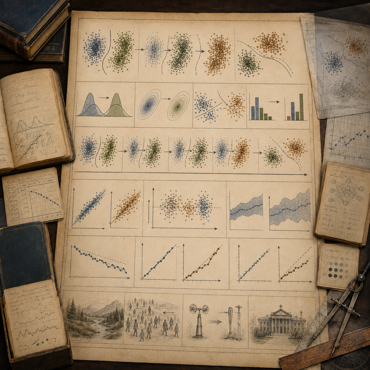
This article explains distribution shift, model decay, covariate shift, label shift, concept drift, domain shift, calibration drift, temporal drift, performance monitoring, retraining, rollback, human review, governance, and representation risk. It emphasizes that models are not static achievements: they are systems operating in changing environments.
Why Distribution Shift and Model Decay Matter
Distribution shift and model decay matter because a model’s development environment is never identical to the world it later enters. The training set is a historical sample. The validation set is a controlled approximation. The test set is a limited evaluation environment. Deployment is different: it is open, changing, interactive, and often adversarial.
A model may fail because users change behavior, because the population changes, because recording systems change, because language evolves, because interventions alter outcomes, because sensors degrade, because policies change, or because the model itself reshapes the environment.
| Development assumption | Deployment reality | Risk |
|---|---|---|
| Training data represent future data. | Future data distributions change. | Performance degrades. |
| Labels mean the same thing over time. | Definitions, policies, or recording practices change. | Label drift and evaluation confusion. |
| Relationships remain stable. | Input-outcome relationships change. | Concept drift. |
| Users do not adapt to the model. | Users learn, evade, game, or rely on the system. | Feedback and strategic drift. |
| Aggregate performance is enough. | Subgroup performance shifts unevenly. | Fairness and safety failures. |
| One approval decision is final. | Deployment conditions keep changing. | Model decay goes unnoticed. |
Model performance is not a permanent property. It is a relationship between a model and a changing environment.
Distribution Shift Defined
Distribution shift occurs when the probability distribution of data changes between training, validation, testing, or deployment. The model learns patterns under one distribution and later encounters another. This can affect features, labels, outcomes, populations, domains, tasks, time periods, contexts, or feedback pathways.
Distribution shift is not always obvious. Aggregate accuracy may remain stable while calibration worsens. Overall performance may look acceptable while one subgroup deteriorates. Input distributions may shift before labels become available. Users may experience failures before dashboards detect them.
| Shift type | What changes | Example |
|---|---|---|
| Covariate shift | Input features change. | New users, new language, new devices, or new contexts appear. |
| Label shift | Outcome frequencies change. | Fraud becomes more common or rare. |
| Concept drift | Relationship between inputs and outcomes changes. | Old predictors no longer indicate risk or success. |
| Domain shift | System moves to a different setting. | Model trained in one hospital is used in another. |
| Temporal shift | Data change over time. | Seasonality, policy changes, economic cycles, or cultural changes. |
| Feedback shift | Model outputs change future data. | Recommendations shape engagement histories. |
A model should be evaluated against the distribution it will face, and monitored when that distribution changes.
Model Decay Defined
Model decay is the deterioration of a model’s usefulness after deployment. It may appear as lower accuracy, worse calibration, higher false positives, higher false negatives, reduced robustness, degraded fairness, safety incidents, increased user complaints, lower trust, or growing dependence on human overrides.
Decay can be gradual or sudden. It may result from natural change, feedback loops, adversarial adaptation, data pipeline changes, policy shifts, new populations, monitoring gaps, or expanding use beyond the original scope.
| Decay signal | Meaning | Possible response |
|---|---|---|
| Accuracy decline | Predictions are less often correct. | Review data shift and retrain if appropriate. |
| Calibration decline | Confidence no longer matches outcomes. | Recalibrate and review uncertainty. |
| Error-pattern change | False positives or false negatives rise. | Check thresholds and subgroup impacts. |
| Fairness gap growth | Performance changes unevenly across groups. | Run disaggregated review and remediation. |
| Override increase | Humans reject model output more often. | Audit reasons and update workflow. |
| Incident increase | Safety or reliability issues accumulate. | Escalate, rollback, or suspend deployment. |
Model decay should be treated as an expected lifecycle risk, not as a rare exception.
Covariate Shift
Covariate shift occurs when the distribution of input features changes while the conditional relationship between features and labels is assumed to remain stable. This can happen when a system reaches new users, enters a new region, handles new devices, faces a new season, or encounters changed behavior.
A model may be asked to make predictions for cases unlike those seen during training. It may still produce confident outputs, but those outputs are less grounded in observed evidence.
| Covariate shift source | How it appears | Monitoring signal |
|---|---|---|
| Population change | New users or groups enter the system. | Feature distribution and subgroup coverage. |
| Device change | Sensor, browser, platform, or interface changes. | Technical metadata shift. |
| Language change | New vocabulary, slang, or formats appear. | Text-feature and embedding drift. |
| Geographic change | Model used in a new region. | Domain and location coverage. |
| Seasonal change | Patterns vary by time of year. | Periodic feature movement. |
| Behavioral adaptation | Users change behavior after deployment. | Interaction and usage-pattern drift. |
Covariate shift is often visible before labels are available, making input monitoring an early warning system.
Label Shift
Label shift occurs when the distribution of outcomes changes. The input patterns may look familiar, but the base rates of classes or outcomes shift. A disease becomes more common. Fraud tactics increase. A moderation category changes frequency. Economic defaults rise. A rare event becomes less rare.
Label shift matters because thresholds, calibration, resource allocation, and performance interpretation depend on outcome prevalence. If base rates change, a model that once worked well may produce misleading probabilities or operational burdens.
| Label shift source | Example | Risk |
|---|---|---|
| Base-rate change | Fraud, disease, or default rate changes. | Thresholds and alerts become misaligned. |
| Policy change | Outcome definition changes. | Old labels no longer match new criteria. |
| Reporting change | More or fewer cases are recorded. | Observed label rate changes without true prevalence change. |
| Intervention change | Actions prevent or produce outcomes. | Labels reflect intervention policy. |
| Seasonal change | Outcomes vary by time period. | Model performance fluctuates predictably. |
| Adversarial change | Bad actors change tactics. | Old labels underrepresent new threats. |
Label shift is not only a statistical issue. It can reflect policy, incentives, access, reporting, and intervention.
Concept Drift
Concept drift occurs when the relationship between inputs and outputs changes. A feature that once predicted an outcome may stop doing so. A pattern that once indicated fraud may become obsolete. A phrase that once signaled one meaning may take on another. A medical or social risk factor may change under new treatment, policy, or behavior.
Concept drift is often harder to detect than covariate shift because the inputs may look similar while the meaning changes.
| Concept drift pattern | Description | Example |
|---|---|---|
| Gradual drift | Relationship changes slowly over time. | Consumer behavior changes across years. |
| Sudden drift | Relationship changes sharply. | Policy change, platform redesign, or crisis event. |
| Recurring drift | Relationship changes cyclically. | Seasonal demand or periodic risk patterns. |
| Incremental drift | One regime gradually replaces another. | Technology adoption changes user behavior. |
| Adversarial drift | Actors intentionally change patterns. | Fraudsters evade detection rules. |
| Semantic drift | Meaning of symbols or language changes. | Words, hashtags, or labels change meaning. |
Concept drift requires outcome monitoring, expert review, and sometimes causal analysis, not only feature-distribution checks.
Domain and Temporal Shift
Domain shift occurs when a model is transferred from one context to another. A model trained in one hospital may fail in another because patient populations, equipment, coding practices, and treatment protocols differ. A model trained on one platform may fail on another because user behavior and interface design differ.
Temporal shift occurs because the same domain changes over time. Even without relocation, populations, technologies, institutions, policies, and language evolve.
| Shift type | Source | Review question |
|---|---|---|
| Domain shift | New institution, geography, platform, or population. | Does the new setting match training conditions? |
| Temporal shift | Time changes the data environment. | How old are the training and validation data? |
| Operational shift | Workflow, policy, or staffing changes. | Does the model still fit the process? |
| Instrument shift | Measurement tools or sensors change. | Are inputs comparable across instruments? |
| Platform shift | Interface or ranking logic changes. | Did user behavior change because design changed? |
| Use-case shift | Model applied beyond intended scope. | Is this deployment covered by the original evaluation? |
A model should not be treated as portable unless portability has been tested.
Calibration Drift
Calibration drift occurs when model confidence no longer matches observed outcomes. A model may remain relatively good at ranking cases while becoming overconfident or underconfident. This is dangerous in decision support, risk scoring, medical prediction, financial forecasting, and safety-critical settings where probability estimates guide action.
Calibration drift can occur because base rates change, labels shift, subgroups change, data quality changes, or the model is used in a new domain.
| Calibration issue | Meaning | Risk |
|---|---|---|
| Overconfidence | Predicted probabilities exceed observed success. | Decision-makers trust outputs too much. |
| Underconfidence | Predicted probabilities are too conservative. | Useful signals may be ignored. |
| Subgroup miscalibration | Calibration differs across groups. | Unequal reliability and fairness risk. |
| Temporal miscalibration | Calibration changes over time. | Old thresholds become unsafe. |
| Threshold misalignment | Decision cutoffs no longer match costs. | Too many or too few interventions. |
| Confidence inflation | System presents certainty without evidence. | Accountability and safety risks increase. |
Monitoring accuracy without calibration can hide serious reliability problems.
Feedback Loops and Decay
Feedback loops can accelerate model decay because outputs change future inputs. A recommender changes what users see. A risk score changes institutional attention. A fraud model changes adversary tactics. A generative model may produce content that later appears in training data. A workplace dashboard changes worker behavior.
In these cases, decay is not only caused by an external world changing. It is partly caused by the model’s own deployment.
| Feedback pathway | How it causes decay | Monitoring need |
|---|---|---|
| Exposure loop | Shown items generate more data than hidden items. | Exposure and opportunity logs. |
| Intervention loop | Actions following predictions alter outcomes. | Intervention and counterfactual review. |
| Adversarial loop | Actors change behavior to evade the model. | Evasion and anomaly monitoring. |
| Recursive data loop | Model outputs enter future training data. | Synthetic and model-mediated data labeling. |
| Metric loop | People optimize measured behavior. | Goodhart-risk review. |
| Reliance loop | Humans change judgment because model exists. | Override, appeal, and automation-bias monitoring. |
Feedback-aware monitoring asks whether the model is degrading because it has changed the system it observes.
Monitoring and Detection
Monitoring should track input data, output distributions, performance, calibration, subgroup results, safety signals, human overrides, incident reports, and use-case expansion. Monitoring is strongest when it combines automated alerts with human review.
Some signals are available immediately, such as input distributions or prediction frequencies. Others require delayed labels, such as true outcomes. Some require qualitative evidence, such as user complaints, audit findings, or expert review.
| Monitoring layer | What it detects | Example signal |
|---|---|---|
| Input monitoring | Covariate shift. | Feature distribution distance. |
| Output monitoring | Prediction-rate changes. | Alert volume or score distribution. |
| Label monitoring | Outcome and base-rate change. | Positive label rate over time. |
| Performance monitoring | Accuracy and error-pattern change. | False positives and false negatives. |
| Calibration monitoring | Confidence reliability. | Expected calibration error or reliability curve. |
| Governance monitoring | Use drift, incidents, and appeals. | Override rate, complaints, and scope changes. |
Monitoring should be designed before deployment, not improvised after failure.
Retraining, Rollback, and Review
Retraining can address model decay, but retraining is not automatically safe. New data may be contaminated by feedback loops, strategic behavior, label changes, or biased recording systems. A decayed model may need recalibration, threshold adjustment, feature review, workflow change, rollback, suspension, or replacement rather than simple retraining.
Rollback is the ability to return to a prior model, rule, threshold, or manual process when monitoring detects unacceptable risk. Review is the governance process that determines what changed and what response is appropriate.
| Response | When useful | Risk if used poorly |
|---|---|---|
| Recalibration | Ranking remains useful but confidence is wrong. | May hide deeper concept drift. |
| Threshold adjustment | Base rates or costs change. | May shift harms across groups. |
| Retraining | New representative data are available. | May learn feedback-shaped or contaminated patterns. |
| Feature review | Inputs changed or degraded. | May miss label or concept drift. |
| Rollback | New model causes incidents or instability. | Old model may also be unsafe. |
| Suspension | Risk exceeds acceptable bounds. | Requires alternative workflow and accountability. |
A responsible model lifecycle includes monitoring triggers, response options, ownership, and authority to stop the system.
Governance and Accountability
Distribution shift and model decay are governance issues because they affect whether a system remains valid, fair, safe, and accountable after deployment. A deployment decision should include monitoring plans, alert thresholds, update procedures, documentation, human review, incident response, and sunset conditions.
Accountability requires knowing who owns the model, who monitors it, who can change it, who can pause it, who receives incident reports, and who is responsible when the deployment environment no longer matches the approved use.
| Governance area | Review question | Documentation |
|---|---|---|
| Deployment scope | Where is the model approved for use? | Use-case and domain statement. |
| Monitoring plan | What signals are tracked after launch? | Monitoring specification. |
| Alert thresholds | When is review triggered? | Threshold and escalation table. |
| Update procedure | How are recalibration, retraining, and rollback governed? | Change-management record. |
| Incident response | How are failures reported and repaired? | Incident and remediation log. |
| Sunset policy | When should the model be retired? | Review and retirement schedule. |
A model that cannot be monitored, updated, paused, or retired is not ready for responsible deployment.
Representation Risk
Representation risk appears when historical evaluation results are presented as if they still describe current system behavior. A benchmark score, test result, validation report, or dashboard metric may reflect a past distribution, not the current deployment environment.
This risk is especially strong when model documentation is treated as a static artifact. The model card, benchmark table, or approval memo may remain unchanged while the world changes around the system.
| Representation risk | How it appears | Review response |
|---|---|---|
| Static performance claims | Old test scores are treated as current evidence. | Add time-stamped monitoring results. |
| Hidden drift | Distribution changes are not documented. | Track input, output, and label distributions. |
| Aggregate stability | Overall metrics hide subgroup decay. | Monitor by group, context, and use case. |
| Deployment overreach | Model used beyond evaluated conditions. | Enforce use boundaries and scope review. |
| Retraining opacity | Model changes without clear documentation. | Version control and change logs. |
| Accountability displacement | Failures blamed on changing data alone. | Assign responsibility for monitoring and response. |
A model’s evidence base should move with the deployment environment, not remain frozen at launch.
Examples of Distribution Shift and Model Decay
The examples below show how shift and decay appear across AI systems, public services, platforms, markets, health, security, and institutional decision-making.
Fraud detection
Fraud patterns change as adversaries learn what the system detects.
Medical prediction
A model trained in one hospital may fail when patient populations, equipment, or coding practices differ.
Recommendation systems
User preferences shift as the system changes what users see.
Credit scoring
Economic cycles change default rates and borrower behavior.
Content moderation
Language, slang, policy definitions, and evasion tactics change over time.
Hiring models
Labor markets, job requirements, and applicant behavior change.
Generative AI evaluation
Benchmarks and usage patterns change as models and users adapt.
Sensor systems
Devices degrade, calibration changes, or new hardware alters data distributions.
Across these examples, the central issue is not whether the model once worked. It is whether the model still works under current conditions.
Mathematics, Computation, and Modeling
Distribution shift can be represented as a difference between training and deployment distributions:
P_{\mathrm{train}}(X,Y) \neq P_{\mathrm{deploy}}(X,Y)
\]
Interpretation: The joint distribution of inputs and outcomes differs between development and deployment.
Covariate shift focuses on changes in input distributions:
P_{\mathrm{train}}(X) \neq P_{\mathrm{deploy}}(X), \qquad P(Y\mid X)\ \text{approximately stable}
\]
Interpretation: Inputs change while the outcome relationship is assumed to remain mostly stable.
Label shift focuses on changes in outcome distributions:
P_{\mathrm{train}}(Y) \neq P_{\mathrm{deploy}}(Y)
\]
Interpretation: Outcome base rates change between training and deployment.
Concept drift occurs when the conditional relationship changes:
P_{\mathrm{train}}(Y\mid X) \neq P_{\mathrm{deploy}}(Y\mid X)
\]
Interpretation: The meaning of inputs changes because their relationship to outcomes changes.
A drift score can be monitored over time:
D_t = D(P_t(X),P_{t-1}(X))
\]
Interpretation: A distance measure \(D_t\) compares current and prior input distributions.
A decay trigger can be based on performance loss:
\mathrm{review}=1 \quad \text{if} \quad M_{\mathrm{baseline}}-M_t>\tau
\]
Interpretation: Review is triggered when current performance \(M_t\) falls far enough below baseline performance.
These formulas show why model monitoring must track both data distributions and model performance. Drift can appear before labels are available, while decay may only become visible after outcomes arrive.
Python Workflow: Distribution Shift and Model Decay Audit
The Python workflow below creates a dependency-light audit for distribution shift and model decay. It simulates deployed model snapshots, computes input drift, label drift, performance decay, calibration drift, subgroup gap change, and review status, then writes reproducible CSV and JSON outputs.
# distribution_shift_model_decay_audit.py
# Dependency-light workflow for drift, decay, calibration, subgroup gaps,
# monitoring triggers, and governance review.

from __future__ import annotations

from dataclasses import asdict, dataclass
from pathlib import Path
from statistics import mean
import csv
import json
from datetime import datetime, timezone

ARTICLE_ROOT = Path(__file__).resolve().parents[1]
TABLES = ARTICLE_ROOT / "outputs" / "tables"
JSON_DIR = ARTICLE_ROOT / "outputs" / "json"


@dataclass(frozen=True)
class DriftDecayConfig:
    article: str = "distribution_shift_and_model_decay"
    input_drift_threshold: float = 0.25
    label_drift_threshold: float = 0.15
    performance_decay_threshold: float = 0.08
    calibration_drift_threshold: float = 0.10
    subgroup_gap_threshold: float = 0.12


def timestamp_utc() -> str:
    return datetime.now(timezone.utc).isoformat()


def write_csv(path: Path, rows: list[dict[str, object]]) -> None:
    path.parent.mkdir(parents=True, exist_ok=True)
    if not rows:
        path.write_text("", encoding="utf-8")
        return
    fieldnames = sorted({key for row in rows for key in row.keys()})
    with path.open("w", newline="", encoding="utf-8") as handle:
        writer = csv.DictWriter(handle, fieldnames=fieldnames, extrasaction="ignore")
        writer.writeheader()
        writer.writerows(rows)


def write_json(path: Path, payload: object) -> None:
    path.parent.mkdir(parents=True, exist_ok=True)
    path.write_text(json.dumps(payload, indent=2, sort_keys=True), encoding="utf-8")


def deployment_snapshots() -> list[dict[str, object]]:
    return [
        {"period": "baseline", "input_drift": 0.00, "label_drift": 0.00, "accuracy": 0.86, "calibration_gap": 0.05, "subgroup_gap": 0.07, "override_rate": 0.04},
        {"period": "month_1", "input_drift": 0.12, "label_drift": 0.04, "accuracy": 0.84, "calibration_gap": 0.06, "subgroup_gap": 0.08, "override_rate": 0.05},
        {"period": "month_2", "input_drift": 0.23, "label_drift": 0.10, "accuracy": 0.81, "calibration_gap": 0.09, "subgroup_gap": 0.11, "override_rate": 0.07},
        {"period": "month_3", "input_drift": 0.31, "label_drift": 0.16, "accuracy": 0.76, "calibration_gap": 0.14, "subgroup_gap": 0.15, "override_rate": 0.11},
        {"period": "month_4", "input_drift": 0.38, "label_drift": 0.19, "accuracy": 0.73, "calibration_gap": 0.18, "subgroup_gap": 0.18, "override_rate": 0.16},
    ]


def audit_snapshot(row: dict[str, object], baseline: dict[str, object], config: DriftDecayConfig) -> dict[str, object]:
    input_drift = float(row["input_drift"])
    label_drift = float(row["label_drift"])
    accuracy = float(row["accuracy"])
    calibration_gap = float(row["calibration_gap"])
    subgroup_gap = float(row["subgroup_gap"])
    override_rate = float(row["override_rate"])
    baseline_accuracy = float(baseline["accuracy"])

    performance_decay = baseline_accuracy - accuracy
    high_input_drift = int(input_drift >= config.input_drift_threshold)
    high_label_drift = int(label_drift >= config.label_drift_threshold)
    high_performance_decay = int(performance_decay >= config.performance_decay_threshold)
    high_calibration_drift = int(calibration_gap >= config.calibration_drift_threshold)
    high_subgroup_gap = int(subgroup_gap >= config.subgroup_gap_threshold)

    decay_risk_score = mean([input_drift, label_drift, max(0.0, performance_decay), calibration_gap, subgroup_gap, override_rate])

    status = "pass"
    if high_input_drift or high_label_drift or high_performance_decay or high_calibration_drift or high_subgroup_gap:
        status = "review"
    if (high_performance_decay and high_calibration_drift) or (high_input_drift and high_subgroup_gap):
        status = "escalate"

    return {
        "period": row["period"],
        "input_drift": round(input_drift, 6),
        "label_drift": round(label_drift, 6),
        "accuracy": round(accuracy, 6),
        "performance_decay": round(performance_decay, 6),
        "calibration_gap": round(calibration_gap, 6),
        "subgroup_gap": round(subgroup_gap, 6),
        "override_rate": round(override_rate, 6),
        "high_input_drift": high_input_drift,
        "high_label_drift": high_label_drift,
        "high_performance_decay": high_performance_decay,
        "high_calibration_drift": high_calibration_drift,
        "high_subgroup_gap": high_subgroup_gap,
        "decay_risk_score": round(decay_risk_score, 6),
        "status": status,
        "interpretation": "Model decay risk rises when data drift, label drift, performance loss, calibration drift, subgroup gaps, or override rates increase.",
    }


def governance_register() -> list[dict[str, str]]:
    return [
        {"item": "deployment_scope", "review_question": "Where is this model approved for use?", "status": "required"},
        {"item": "input_monitoring", "review_question": "How are input distributions tracked?", "status": "required"},
        {"item": "label_monitoring", "review_question": "How are outcome frequencies and definitions tracked?", "status": "required"},
        {"item": "performance_monitoring", "review_question": "How are accuracy and error patterns monitored over time?", "status": "required"},
        {"item": "calibration_monitoring", "review_question": "How is confidence reliability monitored?", "status": "required"},
        {"item": "rollback_plan", "review_question": "When can the model be paused, rolled back, or retired?", "status": "required"},
    ]


def main() -> None:
    config = DriftDecayConfig()
    snapshots = deployment_snapshots()
    baseline = snapshots[0]
    audits = [audit_snapshot(row, baseline, config) for row in snapshots]
    summary = {
        "article": config.article,
        "timestamp_utc": timestamp_utc(),
        "snapshots_reviewed": len(audits),
        "snapshots_passed": sum(1 for row in audits if row["status"] == "pass"),
        "snapshots_requiring_review": sum(1 for row in audits if row["status"] == "review"),
        "snapshots_escalated": sum(1 for row in audits if row["status"] == "escalate"),
        "latest_status": audits[-1]["status"],
        "latest_accuracy": audits[-1]["accuracy"],
        "latest_performance_decay": audits[-1]["performance_decay"],
        "mean_decay_risk_score": round(mean(float(row["decay_risk_score"]) for row in audits), 6),
        "interpretation": "Model deployment should be monitored through input drift, label drift, performance decay, calibration drift, subgroup gaps, override rates, and rollback triggers.",
    }

    write_csv(TABLES / "deployment_snapshots.csv", snapshots)
    write_csv(TABLES / "drift_decay_audit.csv", audits)
    write_csv(TABLES / "drift_decay_governance_register.csv", governance_register())
    write_csv(TABLES / "drift_decay_summary.csv", [summary])

    write_json(JSON_DIR / "drift_decay_config.json", asdict(config))
    write_json(JSON_DIR / "drift_decay_audit.json", audits)
    write_json(JSON_DIR / "drift_decay_summary.json", summary)

    print("Distribution shift and model decay audit complete.")
    print(TABLES / "drift_decay_summary.csv")


if __name__ == "__main__":
    main()
This workflow turns deployment monitoring into a reviewable artifact: drift, decay, calibration, subgroup gaps, override rates, and escalation status are documented together.
R Workflow: Drift and Decay Diagnostics
The R workflow reads the generated CSV outputs, summarizes drift and decay risk, visualizes monitoring signals over time, and writes an additional diagnostic table.
# distribution_shift_model_decay_summary.R
args <- commandArgs(trailingOnly = FALSE)
file_arg <- grep("^--file=", args, value = TRUE)

if (length(file_arg) > 0) {
  script_path <- normalizePath(sub("^--file=", "", file_arg[1]), mustWork = TRUE)
  article_root <- normalizePath(file.path(dirname(script_path), ".."), mustWork = TRUE)
} else {
  article_root <- getwd()
}

setwd(article_root)

tables_dir <- file.path(article_root, "outputs", "tables")
figures_dir <- file.path(article_root, "outputs", "figures")
dir.create(tables_dir, recursive = TRUE, showWarnings = FALSE)
dir.create(figures_dir, recursive = TRUE, showWarnings = FALSE)

audit_path <- file.path(tables_dir, "drift_decay_audit.csv")
summary_path <- file.path(tables_dir, "drift_decay_summary.csv")

if (!file.exists(audit_path)) {
  stop(paste("Missing", audit_path, "Run the Python workflow first."))
}

audit <- read.csv(audit_path, stringsAsFactors = FALSE)
summary <- read.csv(summary_path, stringsAsFactors = FALSE)

png(file.path(figures_dir, "drift_decay_monitoring_signals.png"), width = 1200, height = 850)
score_matrix <- t(as.matrix(audit[, c("input_drift", "label_drift", "performance_decay", "calibration_gap", "subgroup_gap", "override_rate")]))
barplot(score_matrix,
        beside = TRUE,
        names.arg = audit$period,
        las = 2,
        ylim = c(0, 0.45),
        ylab = "Score",
        main = "Distribution Shift and Model Decay Signals")
legend("topleft",
       legend = rownames(score_matrix),
       cex = 0.72,
       bty = "n")
grid()
dev.off()

png(file.path(figures_dir, "drift_decay_status_counts.png"), width = 1000, height = 750)
status_counts <- table(audit$status)
barplot(status_counts,
        ylab = "Count",
        main = "Drift and Decay Audit Status Counts")
grid()
dev.off()

r_summary <- data.frame(
  snapshots_reviewed = summary$snapshots_reviewed[1],
  snapshots_passed = summary$snapshots_passed[1],
  snapshots_requiring_review = summary$snapshots_requiring_review[1],
  snapshots_escalated = summary$snapshots_escalated[1],
  latest_status = summary$latest_status[1],
  latest_accuracy = summary$latest_accuracy[1],
  latest_performance_decay = summary$latest_performance_decay[1],
  mean_decay_risk_score = summary$mean_decay_risk_score[1],
  diagnostic_note = "Model decay should be monitored through data drift, label drift, performance loss, calibration drift, subgroup gaps, override rates, and rollback triggers."
)

write.csv(r_summary, file.path(tables_dir, "r_drift_decay_diagnostic_summary.csv"), row.names = FALSE)
print(r_summary)
The R layer turns drift and decay signals into visible diagnostic summaries that support monitoring, governance, and lifecycle review.
GitHub Repository
The companion repository contains reproducible workflows, synthetic data, audit outputs, calculators, documentation, and multilingual examples for this article.
Complete Code Repository
Companion article folder with Python, R, Julia, SQL, Haskell, C, C++, Fortran, Rust, Go, Java, TypeScript, Prolog, Racket, notebooks, documentation, synthetic teaching data, generated outputs, schemas, calculators, and Canvas-ready workflow artifacts for distribution shift, covariate shift, label shift, concept drift, model decay, calibration drift, subgroup performance, monitoring triggers, retraining review, rollback planning, governance documentation, and responsible algorithmic interpretation.
A Practical Method for Reviewing Model Decay
Model decay should be reviewed as part of the deployment lifecycle, not only after visible failure.
| Step | Review action | Output |
|---|---|---|
| 1 | Define approved deployment scope. | Use-case, domain, and population statement. |
| 2 | Establish baseline distributions and performance. | Baseline monitoring record. |
| 3 | Track inputs, outputs, labels, and calibration. | Monitoring dashboard and audit table. |
| 4 | Review subgroup and context performance. | Disaggregated decay report. |
| 5 | Investigate drift causes. | Change analysis and data-lineage report. |
| 6 | Select response: recalibrate, retrain, adjust threshold, rollback, or suspend. | Governed change record. |
| 7 | Document accountability and future monitoring. | Lifecycle governance record. |
This method treats monitoring as part of model design rather than a maintenance afterthought.
Common Pitfalls
Distribution-shift and model-decay failures often begin when deployment is treated as a static handoff. The system is approved, launched, and then assumed to remain valid. But real-world conditions continue to change.
| Pitfall | Why it matters | Better practice |
|---|---|---|
| Assuming test performance persists | Test data may not match future data. | Use post-deployment monitoring. |
| Monitoring only accuracy | Calibration, fairness, safety, and drift may degrade first. | Track multiple signals. |
| Ignoring subgroup decay | Aggregate metrics can hide uneven failure. | Monitor by group, context, and use case. |
| Retraining automatically | New data may be feedback-shaped or contaminated. | Review data provenance before retraining. |
| No rollback plan | Unsafe models remain active during review. | Define pause, rollback, and manual fallback procedures. |
| Expanding use silently | Model is used outside validated scope. | Require scope-change approval. |
A model that performs well once can still become unreliable later.
Why Deployment Requires Monitoring
Distribution shift and model decay reveal a basic truth about algorithmic systems: deployment is not the end of evaluation. It is the beginning of a new phase in which the model interacts with a changing world.
A model’s inputs, labels, outcomes, users, institutions, and feedback pathways can all change after launch. These changes can degrade accuracy, calibration, fairness, safety, and usefulness. They can also make old performance claims misleading.
Responsible computational reasoning therefore requires lifecycle governance. Models need baseline records, monitoring signals, drift alerts, disaggregated review, calibration checks, incident reporting, retraining controls, rollback plans, and sunset policies. A model remains trustworthy only if the evidence supporting it remains current.
Related Articles
- Feedback Loops in Algorithmic Systems
- Proxy Variables and Measurement Error
- Training, Testing, and Generalization
- Overfitting, Underfitting, and Model Error
Further Reading
- Quiñonero-Candela, J. et al. (eds.) (2009) Dataset Shift in Machine Learning. Cambridge, MA: MIT Press.
- Moreno-Torres, J.G. et al. (2012) ‘A unifying view on dataset shift in classification’, Pattern Recognition, 45(1), pp. 521–530.
- Gama, J. et al. (2014) ‘A survey on concept drift adaptation’, ACM Computing Surveys, 46(4), Article 44.
- Lu, J. et al. (2019) ‘Learning under concept drift: a review’, IEEE Transactions on Knowledge and Data Engineering, 31(12), pp. 2346–2363.
- Ovadia, Y. et al. (2019) ‘Can you trust your model’s uncertainty? Evaluating predictive uncertainty under dataset shift’, Advances in Neural Information Processing Systems.
- National Institute of Standards and Technology (2024) Artificial Intelligence Risk Management Framework. Gaithersburg, MD: NIST.
References
- Gama, J., Žliobaitė, I., Bifet, A., Pechenizkiy, M. and Bouchachia, A. (2014) ‘A survey on concept drift adaptation’, ACM Computing Surveys, 46(4), Article 44. Available at: https://dl.acm.org/doi/10.1145/2523813.
- Lu, J., Liu, A., Dong, F., Gu, F., Gama, J. and Zhang, G. (2019) ‘Learning under concept drift: a review’, IEEE Transactions on Knowledge and Data Engineering, 31(12), pp. 2346–2363. Available at: https://ieeexplore.ieee.org/document/8496795.
- Moreno-Torres, J.G., Raeder, T., Alaiz-Rodríguez, R., Chawla, N.V. and Herrera, F. (2012) ‘A unifying view on dataset shift in classification’, Pattern Recognition, 45(1), pp. 521–530. Available at: https://doi.org/10.1016/j.patcog.2011.06.019.
- National Institute of Standards and Technology (2024) Artificial Intelligence Risk Management Framework. Gaithersburg, MD: NIST. Available at: https://www.nist.gov/itl/ai-risk-management-framework.
- Ovadia, Y., Fertig, E., Ren, J., Nado, Z., Sculley, D., Nowozin, S., Dillon, J., Lakshminarayanan, B. and Snoek, J. (2019) ‘Can you trust your model’s uncertainty? Evaluating predictive uncertainty under dataset shift’, Advances in Neural Information Processing Systems. Available at: https://papers.nips.cc/paper_files/paper/2019/hash/8558cb408c1d76621371888657d2eb1d-Abstract.html.
- Quiñonero-Candela, J., Sugiyama, M., Schwaighofer, A. and Lawrence, N.D. (eds.) (2009) Dataset Shift in Machine Learning. Cambridge, MA: MIT Press. Available at: https://mitpress.mit.edu/9780262170055/dataset-shift-in-machine-learning/.