
Last Updated July 6, 2026
Dimensionality Reduction in High-Dimensional Data shows how linear algebra turns complex datasets into lower-dimensional structure without pretending the compression is neutral. Modern datasets often contain many variables: sensors, images, documents, embeddings, biological measurements, economic indicators, infrastructure records, behavioral logs, climate variables, and machine-learning features. High dimensionality can reveal detail, but it can also create noise, redundancy, instability, sparsity, overfitting, and interpretation problems.
This article continues Part X of the Linear Algebra for Systems Modeling series by applying matrix methods to dimensionality reduction: feature matrices, centering, scaling, covariance, correlation, projection, PCA, SVD, singular values, principal components, explained variance, reconstruction error, latent dimensions, noise filtering, visualization, model compression, validation, leakage risk, interpretability, uncertainty, and responsible use.
The central modeling question is not only “Can the data be reduced?” It is “What structure is preserved, what is lost, and what claims can responsibly be made after high-dimensional data have been projected into fewer dimensions?”
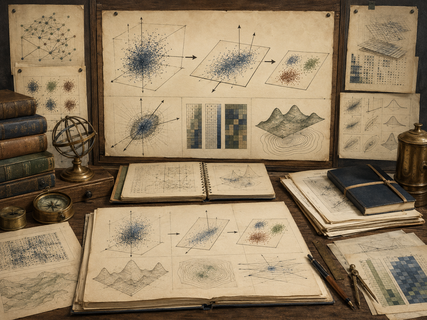
Dimensionality reduction begins with a feature matrix. Rows represent observations. Columns represent variables, features, measurements, tokens, signals, indicators, or embeddings. The goal is to represent the data in fewer dimensions while retaining useful structure. In linear methods such as PCA and SVD, this means finding directions, subspaces, or factors that capture major patterns of variation.
The method can clarify structure, reduce noise, improve visualization, compress models, speed computation, and support downstream analysis. It can also hide minority patterns, erase rare signals, mix variables into opaque components, leak information across train-test boundaries, or turn an exploratory projection into an unsupported explanation. Dimensionality reduction is therefore both a mathematical tool and an interpretive responsibility.
Why Dimensionality Reduction Matters
Dimensionality reduction matters because high-dimensional data are difficult to inspect, visualize, validate, and model directly. Many variables may be redundant. Some features may be noisy. Some may be strongly correlated. Some may measure the same underlying process. Some may reflect measurement artifacts. Some may be meaningful only when combined with others.
Linear algebra provides tools for finding structured lower-dimensional representations. PCA identifies orthogonal directions of maximum variance. SVD decomposes a matrix into singular vectors and singular values. Projection maps high-dimensional observations into a lower-dimensional subspace. Reconstruction error measures what is lost when the lower-dimensional representation is used to approximate the original data.
| High-dimensional problem | Linear algebra tool | What it can clarify |
|---|---|---|
| Too many variables to inspect directly | Projection | Lower-dimensional summaries of observations. |
| Correlated features | PCA or SVD | Dominant directions of shared variation. |
| Noisy measurements | Truncated components | Approximate signal while suppressing smaller variation. |
| Large matrix computation | Low-rank approximation | Compact representation for storage or modeling. |
| Visualization challenge | Two- or three-dimensional embedding | Exploratory visual structure. |
| Downstream model instability | Dimension reduction before modeling | Reduced feature space and potential regularization. |
The value of dimensionality reduction is disciplined simplification. The danger is forgetting that simplification changes the evidence.
Case Study Framing
This case study uses a synthetic high-dimensional dataset with observations and features. The workflow centers the data, scales the features, applies PCA through SVD, selects a reduced number of components, measures explained variance, reconstructs the data, and records interpretation warnings.
The case asks:
- How does a feature matrix become a geometric object?
- Why do centering and scaling change the result?
- How do PCA and SVD identify lower-dimensional structure?
- How should explained variance and reconstruction error be interpreted?
- How can dimensionality reduction support modeling without leaking information?
- What should be documented before reduced dimensions guide decisions?
| Case element | Modeling meaning | Interpretive warning |
|---|---|---|
| Observation | Row of the feature matrix. | Rows may represent people, assets, documents, regions, time periods, or systems with different ethical stakes. |
| Feature | Column of the feature matrix. | Features may encode measurement choices, proxies, noise, or historical bias. |
| Centering | Subtracting feature means. | Changes the origin and makes variation relative to the sample mean. |
| Scaling | Normalizing feature units or variance. | Changes which variables dominate the projection. |
| Component | Direction of variation or latent axis. | Components are mathematical mixtures, not automatically meaningful causes. |
| Reduced representation | Lower-dimensional coordinates. | Compression may lose rare, local, nonlinear, or minority patterns. |
The synthetic case keeps the computation visible. Real systems require stronger data governance, validation, feature review, and interpretation boundaries.
Feature Matrices and High-Dimensional Structure
A high-dimensional dataset can be represented as a matrix \(X\), where each row is an observation and each column is a feature. If there are \(n\) observations and \(p\) features, then \(X\) is an \(n \times p\) matrix.
X \in \mathbb{R}^{n \times p}
\]
Interpretation: A feature matrix represents observations as points in a \(p\)-dimensional feature space.
High-dimensional structure may come from meaningful latent processes, redundant measurement, correlated variables, repeated signals, noise, artifacts, or data-collection design. Dimensionality reduction does not know which is which automatically. It finds mathematical structure that must be interpreted.
| Feature matrix context | Rows may represent | Columns may represent |
|---|---|---|
| Infrastructure monitoring | Assets, sensors, facilities, regions, or time periods. | Condition indicators, loads, failures, inspections, climate exposures. |
| Text analysis | Documents, paragraphs, articles, or queries. | Terms, topics, embeddings, metadata, or semantic features. |
| Public health | Patients, regions, cohorts, or time periods. | Risk factors, symptoms, outcomes, exposure measures. |
| Economics | Industries, countries, households, firms, or years. | Indicators, transactions, prices, labor, trade, demand variables. |
| Machine learning | Training examples. | Input features, transformed variables, embeddings, engineered predictors. |
| Science and engineering | Experiments, simulations, samples, or systems. | Measurements, parameters, outputs, signals, or derived features. |
Before reducing dimension, the matrix must be understood as data about something. Rows and columns carry meaning, provenance, and risk.
Centering, Scaling, and Preprocessing
Centering subtracts the feature mean. Scaling changes the relative magnitude of features. These steps are not technical details. They define what variation the dimensionality reduction method will treat as important.
\tilde{X}_{ij}=X_{ij}-\bar{x}_j
\]
Interpretation: Centering makes each feature’s values relative to its sample mean.
Z_{ij}=\frac{X_{ij}-\bar{x}_j}{s_j}
\]
Interpretation: Standardization divides centered values by feature scale, often the sample standard deviation.
If features are measured in different units, unscaled PCA may be dominated by high-variance or high-unit features. If all features are standardized, each feature receives equal variance weight even when some scales are substantively meaningful. Neither choice is universally correct.
| Preprocessing choice | Effect | Review question |
|---|---|---|
| No centering | Components may reflect means or offsets. | Is the origin meaningful? |
| Mean centering | Components reflect variation around feature means. | Are means stable and representative? |
| Standardization | Features contribute according to standardized variance. | Should all features receive equal variance scale? |
| Robust scaling | Reduces influence of outliers. | Are outliers errors or important events? |
| Log transformation | Compresses skewed positive variables. | Does the transformation preserve meaningful relationships? |
| Missing-data imputation | Completes matrix for decomposition. | Does imputation add structure or hide missingness? |
Preprocessing decisions should be documented with the same seriousness as the reduction method itself.
Covariance, Correlation, and Variation
PCA is often described through covariance. For centered data, the covariance matrix summarizes how features vary together.
S=\frac{1}{n-1}\tilde{X}^T\tilde{X}
\]
Interpretation: The covariance matrix summarizes pairwise feature variation in centered data.
If standardized data are used, PCA is related to the correlation matrix rather than the raw covariance matrix. This changes the meaning of the components. Covariance-based PCA preserves original variance scale. Correlation-based PCA emphasizes standardized relationships.
| Matrix | Used when | Interpretive warning |
|---|---|---|
| Covariance matrix | Feature units and variances are substantively meaningful. | Large-scale features can dominate components. |
| Correlation matrix | Features should be compared after standardization. | Equalizing variance may overemphasize noisy small-scale features. |
| Centered feature matrix | Working directly with PCA or SVD. | Mean structure is removed and must be interpreted accordingly. |
| Scaled feature matrix | Units differ or standardized comparison is desired. | Scaling can change component order and loading interpretation. |
| Gram matrix | Comparing observations rather than features. | May become expensive or unstable in large datasets. |
| Kernel matrix | Nonlinear similarity representation. | Interpretation depends on kernel choice and hyperparameters. |
Variation is not automatically importance. A high-variance direction may be meaningful, noisy, biased, or merely dominant because of measurement scale.
Projection and Subspaces
Dimensionality reduction often means projecting data onto a lower-dimensional subspace. If \(W_k\) contains \(k\) basis directions, then the reduced representation is:
Y=XW_k
\]
Interpretation: The reduced matrix \(Y\) contains lower-dimensional coordinates of the original observations.
A projection preserves some structure and discards other structure. In PCA, the chosen subspace maximizes variance captured under orthogonality constraints. But a projection that preserves variance may not preserve class separation, causal relationships, rare events, fairness-relevant structure, interpretability, or downstream predictive performance.
| Projection preserves | Projection may distort | Review method |
|---|---|---|
| Dominant linear variation | Low-variance but important signals. | Inspect reconstruction error and domain-relevant residuals. |
| Global structure | Local neighborhoods. | Compare neighborhood preservation where relevant. |
| Orthogonal component coordinates | Original feature meanings. | Review loadings and component interpretation. |
| Large-scale patterns | Minority or rare patterns. | Disaggregate validation across groups and regimes. |
| Compact representation | Measurement provenance. | Keep preprocessing and feature documentation attached. |
| Computational efficiency | Uncertainty and model limits. | Attach validation and sensitivity results to outputs. |
Projection is not just smaller data. It is transformed data.
Principal Component Analysis
Principal Component Analysis identifies orthogonal directions that capture maximum variance in the data. The first principal component captures the largest possible variance along a single direction. The second captures the largest remaining variance subject to orthogonality, and so on.
w_1=\arg\max_{\|w\|=1} \operatorname{Var}(Xw)
\]
Interpretation: The first principal component direction maximizes projected variance among unit vectors.
PCA is useful for reducing redundancy, visualizing dominant variation, identifying latent structure, preprocessing for modeling, and compressing high-dimensional data. But PCA components are mathematical directions. They are not automatically causal factors, natural categories, or interpretable concepts.
| PCA output | Meaning | Interpretive warning |
|---|---|---|
| Component direction | Linear combination of original features. | May mix unrelated mechanisms or measurement artifacts. |
| Component score | Observation coordinate along a component. | Score depends on preprocessing and component orientation. |
| Loading | Feature contribution to component direction. | Large loading is not automatically causal importance. |
| Explained variance | Variance captured by a component. | Variance is not the same as meaning, fairness, or predictive value. |
| Reduced representation | Coordinates in lower-dimensional space. | Can hide patterns not aligned with top components. |
| Reconstruction | Approximation of original data from selected components. | Low average error can hide high error for subgroups or rare cases. |
PCA is a linear approximation method. Its results should be interpreted as structure in the data representation, not as direct structure in the world unless validated by domain evidence.
Singular Value Decomposition
Singular Value Decomposition decomposes a matrix into left singular vectors, singular values, and right singular vectors:
X=U\Sigma V^T
\]
Interpretation: SVD expresses a data matrix as orthogonal observation patterns, singular values, and orthogonal feature directions.
For centered data, PCA can be computed through SVD. The right singular vectors correspond to principal directions. Singular values determine explained variance. Truncating the SVD gives a low-rank approximation.
X_k=U_k\Sigma_kV_k^T
\]
Interpretation: A rank-\(k\) approximation keeps the top \(k\) singular components and discards the rest.
SVD is especially important for large-scale computation, latent semantic analysis, matrix approximation, recommendation systems, scientific computing, signal processing, and numerical linear algebra.
| SVD object | Role | Interpretive warning |
|---|---|---|
| \(U\) | Observation-side singular vectors. | Observation patterns may not correspond to natural groups. |
| \(\Sigma\) | Singular values ordered by magnitude. | Large singular value may reflect scale, redundancy, or artifact. |
| \(V\) | Feature-side singular vectors. | Feature directions are mixtures of original variables. |
| \(X_k\) | Low-rank approximation. | Approximation discards residual structure. |
| Truncation | Compression and noise reduction. | Small components may contain important rare signals. |
| Numerical method | Stable computation for matrix factorization. | Large-scale approximations require error checks. |
SVD is a mathematical workhorse because it connects geometry, approximation, variance, computation, and data compression in one decomposition.
Explained Variance and Component Selection
Explained variance is often used to decide how many components to keep. For PCA computed through SVD, the variance associated with each component is related to the squared singular values.
\text{Explained variance ratio}_j=\frac{\sigma_j^2}{\sum_{\ell}\sigma_\ell^2}
\]
Interpretation: The explained variance ratio measures the share of total variance captured by component \(j\).
A common rule is to keep enough components to explain a chosen percentage of variance. This is useful but incomplete. A component may explain little variance yet preserve an important rare event, minority subgroup, anomaly, or decision-relevant distinction. A component may explain much variance but mostly reflect scale, noise, or collection bias.
| Selection method | Strength | Risk |
|---|---|---|
| Cumulative explained variance | Simple and transparent. | May ignore low-variance important structure. |
| Scree plot | Shows diminishing returns visually. | Elbow choice can be subjective. |
| Cross-validation | Connects component count to downstream performance. | Must avoid leakage and overfitting. |
| Reconstruction error | Measures approximation quality. | Average error can hide subgroup error. |
| Domain threshold | Connects selection to purpose. | Requires explicit justification. |
| Stability analysis | Tests robustness across samples or perturbations. | Can be computationally expensive. |
Component selection should be tied to modeling purpose, not only to a single variance threshold.
Reconstruction Error and Information Loss
A reduced representation can be used to reconstruct an approximation of the original data. Reconstruction error measures how much information is lost under the chosen low-dimensional representation.
\|X-X_k\|_F
\]
Interpretation: The Frobenius norm of the residual matrix measures total reconstruction error.
Low reconstruction error can support compression and denoising, but it does not prove that all meaningful structure has been preserved. Reconstruction error is often an average or aggregate measure. It can hide errors concentrated in specific observations, subgroups, time periods, sectors, regions, or rare conditions.
| Error view | Clarifies | Can hide |
|---|---|---|
| Total reconstruction error | Overall approximation loss. | Where errors are concentrated. |
| Per-feature error | Variables poorly preserved. | Observation-level consequences. |
| Per-observation error | Cases poorly approximated. | Feature-specific distortion. |
| Subgroup error | Uneven preservation across groups. | Unlabeled or unobserved groups. |
| Time-period error | Temporal instability. | Cross-sectional heterogeneity. |
| Downstream task error | Effect on prediction, classification, retrieval, or clustering. | Interpretability and causal meaning. |
Information loss is not only mathematical. It can also be practical, institutional, ethical, and interpretive.
Noise Filtering, Signal, and Rare Patterns
Dimensionality reduction is often used to separate signal from noise. Truncated PCA or SVD can remove smaller components that may reflect measurement error, random variation, or idiosyncratic fluctuations. But smaller components are not always noise.
Rare but important structure may live in lower-variance directions: equipment failure precursors, fraud patterns, emerging disease signals, local climate extremes, minority-language text clusters, underrepresented populations, unusual infrastructure dependencies, or early warning indicators. A reduction method optimized for dominant variance may suppress these signals.
| Pattern type | Reduction may help by | Reduction may harm by |
|---|---|---|
| Redundant measurement | Combining correlated variables. | Making component interpretation opaque. |
| Random noise | Suppressing low-variance instability. | Discarding weak but real signal. |
| Rare event | Sometimes separating anomaly structure. | Dropping low-frequency patterns. |
| Minority pattern | Revealing hidden clusters in some cases. | Compressing patterns into dominant-group structure. |
| Measurement artifact | Exposing shared artifact directions. | Treating artifact as meaningful component. |
| Latent factor | Approximating common underlying variation. | Overinterpreting factor as real mechanism. |
Noise filtering requires domain judgment. The smallest components are not automatically disposable, and the largest components are not automatically meaningful.
Visualization and Cluster Interpretation
Dimensionality reduction is often used for visualization. A two-dimensional projection can help analysts see structure that would be impossible to inspect in the original feature space. But visualization is especially vulnerable to overinterpretation.
PCA visualizations preserve dominant linear variance. Nonlinear methods such as t-SNE or UMAP can preserve certain local neighborhood relationships and reveal cluster-like structure, but distances, gaps, and cluster shapes in the visualization may not have straightforward global meaning. Parameters can strongly influence the picture.
| Visualization claim | Safer interpretation | Warning |
|---|---|---|
| “These points are close.” | They are close under this projection and preprocessing. | Original-space distance may differ. |
| “These clusters are real.” | The projection suggests possible structure. | Clustering should be validated separately. |
| “This axis means X.” | The axis may reflect a mixture of features. | Component loadings and domain evidence are needed. |
| “Group A is separated from Group B.” | The projection separates groups under chosen assumptions. | Separation may depend on scaling, features, or parameters. |
| “This point is an outlier.” | The point appears unusual in the reduced view. | Outlier status requires original-space and domain review. |
| “The model discovered categories.” | The projection suggests candidate patterns. | Discovery language requires validation and uncertainty review. |
Reduced-dimensional visualizations are exploratory evidence. They should prompt questions, not end them.
Modeling Risk, Leakage, and Validation
Dimensionality reduction often appears inside machine-learning pipelines. This introduces a serious risk: data leakage. If PCA or scaling is fit on the full dataset before train-test splitting or cross-validation, information from the test set can influence the reduced representation. This can inflate performance estimates.
The correct workflow fits preprocessing and dimensionality reduction only on training data, then applies the learned transformation to validation or test data. Cross-validation should include the reduction step inside each fold.
| Workflow step | Safe practice | Leakage risk |
|---|---|---|
| Train-test split | Split before fitting scaling or PCA. | Fitting on all data leaks test distribution. |
| Scaling | Fit means and scales on training data only. | Test data influence preprocessing parameters. |
| PCA or SVD | Fit components on training data only. | Test data influence component directions. |
| Cross-validation | Include reduction inside each fold pipeline. | Global preprocessing contaminates fold estimates. |
| Component selection | Select using training or nested validation only. | Choosing components based on test performance overfits evaluation. |
| Reporting | Report preprocessing, component count, validation method, and uncertainty. | Reduced-space results appear more robust than they are. |
Dimensionality reduction should be validated for its intended use: visualization, compression, denoising, clustering, retrieval, prediction, anomaly detection, or explanation. Each use requires different evidence.
Mathematical Deepening
This section adds a more formal layer. Dimensionality reduction connects feature matrices, centering, scaling, covariance matrices, eigendecomposition, singular value decomposition, orthogonal projection, low-rank approximation, explained variance, reconstruction error, numerical stability, validation, and responsible interpretation.
Representation Review
Observation Semantics
Define what rows represent: people, assets, documents, regions, time periods, sensors, cases, simulations, or systems.
Feature Semantics
State what columns measure, how they were collected, whether they are proxies, and what units or scales they use.
Preprocessing Semantics
Document centering, scaling, imputation, transformation, filtering, and outlier handling.
Reduction Purpose
Record whether the reduction supports visualization, compression, denoising, clustering, prediction, retrieval, or explanation.
Matrix Review
Feature Matrix
Use \(X\) to represent observations by features in a structured rectangular dataset.
Centered Matrix
Use \(\tilde{X}\) to represent data after subtracting feature means.
Covariance Matrix
Use \(S=\frac{1}{n-1}\tilde{X}^T\tilde{X}\) to summarize feature variation.
SVD
Use \(X=U\Sigma V^T\) to decompose observations, singular values, and feature directions.
Diagnostic Review
Explained Variance
Inspect component-level and cumulative explained variance without treating variance as automatic meaning.
Reconstruction Error
Measure aggregate, per-feature, per-observation, and subgroup reconstruction error.
Stability Review
Test whether components and downstream results remain stable across samples, perturbations, or time periods.
Leakage Review
Ensure scaling and component fitting happen inside training folds or training data only.
Responsibility Review
Interpretability
Review component loadings, feature contributions, and whether component labels are justified.
Rare Pattern Preservation
Check whether rare, minority, local, or high-stakes patterns are lost in the reduced representation.
Validation
Connect the reduced representation to task-specific evidence, not only mathematical compression metrics.
Decision Boundary
Attach preprocessing choices, component count, uncertainty, validation status, and stop-use conditions to outputs.
Case Study Workflow
A responsible dimensionality reduction workflow moves from data representation to preprocessing, decomposition, component selection, validation, and interpretation limits.
1. Define Rows and Columns
Specify what observations and features represent, how they were measured, and what risks or proxies they contain.
2. Preprocess Carefully
Document centering, scaling, imputation, transformation, filtering, and outlier handling before decomposition.
3. Apply PCA or SVD
Compute principal directions, singular values, component scores, explained variance, and low-rank approximation.
4. Select Components
Choose component count using variance, reconstruction error, stability, task performance, and domain purpose.
5. Validate Reduced Structure
Check reconstruction loss, subgroup error, rare-pattern preservation, leakage risk, and downstream performance.
6. Interpret Responsibly
Explain what was preserved, what was discarded, what assumptions shaped the projection, and what decisions require additional review.
This workflow treats dimensionality reduction as structured approximation, not as neutral simplification.
Computation and Reproducible Workflows
Computational workflows for dimensionality reduction should document feature definitions, preprocessing choices, centering and scaling parameters, decomposition method, component count, explained variance, reconstruction error, stability checks, leakage controls, validation method, subgroup review, rare-pattern review, and responsible-use warnings.
The companion repository treats dimensionality reduction as an auditable modeling workflow. Python, R, Julia, SQL, Haskell, C, C++, Fortran, Rust, Go, notebooks, schemas, generated outputs, Canvas artifacts, advanced reports, and calculators each support a different layer of matrix construction, PCA/SVD computation, reconstruction review, validation, and responsible interpretation.
For this article, the computational examples build a synthetic feature matrix, standardize the data, compute a covariance matrix, estimate principal components, reduce to two dimensions, reconstruct the data, calculate explained variance and reconstruction error, and export a governance-ready audit report.
Python Workflow: Dimensionality Reduction Audit
The Python workflow below creates a synthetic feature matrix, standardizes it, computes PCA through eigenanalysis of the covariance matrix, reduces to two components, measures explained variance and reconstruction error, and exports a structured audit record.
from __future__ import annotations

from dataclasses import asdict, dataclass
from pathlib import Path
import csv
import json
import math


@dataclass(frozen=True)
class DimensionalityReductionAudit:
    workflow_name: str
    scenario_name: str
    observation_count: int
    feature_count: int
    retained_components: int
    cumulative_explained_variance: float
    reconstruction_rmse: float
    dominant_component_feature: str
    preprocessing_summary: str
    validation_warning: str
    interpretation_warning: str


FEATURES = ["load", "temperature", "vibration", "pressure", "latency"]

DATA = [
    [80.0, 31.0, 0.42, 101.0, 14.0],
    [82.0, 32.0, 0.45, 100.0, 15.0],
    [78.0, 30.0, 0.41, 102.0, 13.0],
    [95.0, 37.0, 0.62, 96.0, 22.0],
    [97.0, 38.0, 0.65, 95.0, 24.0],
    [94.0, 36.0, 0.60, 97.0, 21.0],
    [70.0, 28.0, 0.35, 104.0, 11.0],
    [72.0, 29.0, 0.36, 103.0, 12.0],
]


def mean(values: list[float]) -> float:
    return sum(values) / len(values)


def transpose(matrix: list[list[float]]) -> list[list[float]]:
    return [list(col) for col in zip(*matrix)]


def standardize(matrix: list[list[float]]) -> tuple[list[list[float]], list[float], list[float]]:
    cols = transpose(matrix)
    means = [mean(col) for col in cols]
    scales = []
    for col, mu in zip(cols, means):
        variance = sum((value - mu) ** 2 for value in col) / (len(col) - 1)
        scales.append(math.sqrt(variance))
    standardized = [
        [(row[j] - means[j]) / scales[j] for j in range(len(row))]
        for row in matrix
    ]
    return standardized, means, scales


def covariance(matrix: list[list[float]]) -> list[list[float]]:
    n = len(matrix)
    p = len(matrix[0])
    return [
        [
            sum(matrix[i][a] * matrix[i][b] for i in range(n)) / (n - 1)
            for b in range(p)
        ]
        for a in range(p)
    ]


def matvec(matrix: list[list[float]], vector: list[float]) -> list[float]:
    return [sum(row[j] * vector[j] for j in range(len(vector))) for row in matrix]


def dot(a: list[float], b: list[float]) -> float:
    return sum(x * y for x, y in zip(a, b))


def norm(vector: list[float]) -> float:
    return math.sqrt(dot(vector, vector))


def outer(a: list[float], b: list[float]) -> list[list[float]]:
    return [[x * y for y in b] for x in a]


def subtract_matrix(A: list[list[float]], B: list[list[float]]) -> list[list[float]]:
    return [[A[i][j] - B[i][j] for j in range(len(A[0]))] for i in range(len(A))]


def power_iteration(matrix: list[list[float]], iterations: int = 200) -> tuple[float, list[float]]:
    p = len(matrix)
    vector = [1.0 / math.sqrt(p) for _ in range(p)]
    for _ in range(iterations):
        nxt = matvec(matrix, vector)
        length = norm(nxt)
        if length == 0:
            break
        vector = [value / length for value in nxt]
    eigenvalue = dot(vector, matvec(matrix, vector))
    return eigenvalue, vector


def top_eigenpairs_symmetric(matrix: list[list[float]], k: int) -> list[tuple[float, list[float]]]:
    working = [row[:] for row in matrix]
    pairs = []
    for _ in range(k):
        eigenvalue, vector = power_iteration(working)
        pairs.append((eigenvalue, vector))
        working = subtract_matrix(working, [[eigenvalue * cell for cell in row] for row in outer(vector, vector)])
    return pairs


def project(matrix: list[list[float]], components: list[list[float]]) -> list[list[float]]:
    return [[dot(row, component) for component in components] for row in matrix]


def reconstruct(scores: list[list[float]], components: list[list[float]]) -> list[list[float]]:
    p = len(components[0])
    return [
        [sum(score[j] * components[j][feature] for j in range(len(components))) for feature in range(p)]
        for score in scores
    ]


def rmse(A: list[list[float]], B: list[list[float]]) -> float:
    count = len(A) * len(A[0])
    return math.sqrt(sum((A[i][j] - B[i][j]) ** 2 for i in range(len(A)) for j in range(len(A[0]))) / count)


def build_audit() -> DimensionalityReductionAudit:
    standardized, _, _ = standardize(DATA)
    cov = covariance(standardized)
    retained = 2
    eigenpairs = top_eigenpairs_symmetric(cov, retained)
    eigenvalues = [pair[0] for pair in eigenpairs]
    components = [pair[1] for pair in eigenpairs]
    total_variance = sum(cov[i][i] for i in range(len(cov)))
    cumulative_explained = sum(eigenvalues) / total_variance

    scores = project(standardized, components)
    reconstructed = reconstruct(scores, components)
    reconstruction_error = rmse(standardized, reconstructed)

    first_component = components[0]
    dominant_index = max(range(len(FEATURES)), key=lambda i: abs(first_component[i]))

    return DimensionalityReductionAudit(
        workflow_name="dimensionality_reduction_audit",
        scenario_name="synthetic_high_dimensional_sensor_feature_matrix",
        observation_count=len(DATA),
        feature_count=len(FEATURES),
        retained_components=retained,
        cumulative_explained_variance=round(cumulative_explained, 12),
        reconstruction_rmse=round(reconstruction_error, 12),
        dominant_component_feature=FEATURES[dominant_index],
        preprocessing_summary="Features were centered and standardized before covariance-based PCA.",
        validation_warning=(
            "Component selection should be checked against reconstruction error, stability, subgroup error, "
            "rare-pattern preservation, and downstream task performance."
        ),
        interpretation_warning=(
            "Principal components are mathematical directions of variation. They are not automatically causal factors, "
            "natural categories, or decision-ready explanations. Scaling, feature choice, missing data, leakage controls, "
            "and validation evidence must remain attached to the reduced representation."
        ),
    )


def write_outputs(output_dir: Path) -> None:
    (output_dir / "tables").mkdir(parents=True, exist_ok=True)
    (output_dir / "json").mkdir(parents=True, exist_ok=True)
    (output_dir / "reports").mkdir(parents=True, exist_ok=True)

    audit = build_audit()
    row = asdict(audit)

    with (output_dir / "tables" / "dimensionality_reduction_audit.csv").open(
        "w", newline="", encoding="utf-8"
    ) as handle:
        writer = csv.DictWriter(handle, fieldnames=list(row.keys()))
        writer.writeheader()
        writer.writerow(row)

    (output_dir / "json" / "dimensionality_reduction_audit.json").write_text(
        json.dumps(row, indent=2, sort_keys=True),
        encoding="utf-8",
    )

    report = [
        "# Dimensionality Reduction Audit",
        "",
        f"- Workflow: {audit.workflow_name}",
        f"- Scenario: {audit.scenario_name}",
        f"- Observation count: {audit.observation_count}",
        f"- Feature count: {audit.feature_count}",
        f"- Retained components: {audit.retained_components}",
        f"- Cumulative explained variance: {audit.cumulative_explained_variance}",
        f"- Reconstruction RMSE: {audit.reconstruction_rmse}",
        f"- Dominant first-component feature: {audit.dominant_component_feature}",
        "",
        audit.preprocessing_summary,
        "",
        audit.validation_warning,
        "",
        audit.interpretation_warning,
    ]

    (output_dir / "reports" / "dimensionality_reduction_audit.md").write_text(
        "\\n".join(report) + "\\n",
        encoding="utf-8",
    )


if __name__ == "__main__":
    write_outputs(Path("outputs"))
    print("Dimensionality reduction audit complete.")
This workflow keeps preprocessing, component selection, explained variance, reconstruction error, validation warning, and interpretation boundary together in one auditable artifact.
R Workflow: PCA and Reconstruction Review
R can support the same case study by standardizing a feature matrix, applying PCA, reducing the data, reconstructing the standardized matrix, measuring error, and exporting a responsible modeling audit.
features <- c("load", "temperature", "vibration", "pressure", "latency")

X <- matrix(
  c(
    80.0, 31.0, 0.42, 101.0, 14.0,
    82.0, 32.0, 0.45, 100.0, 15.0,
    78.0, 30.0, 0.41, 102.0, 13.0,
    95.0, 37.0, 0.62, 96.0, 22.0,
    97.0, 38.0, 0.65, 95.0, 24.0,
    94.0, 36.0, 0.60, 97.0, 21.0,
    70.0, 28.0, 0.35, 104.0, 11.0,
    72.0, 29.0, 0.36, 103.0, 12.0
  ),
  ncol = length(features),
  byrow = TRUE
)

colnames(X) <- features

pca <- prcomp(X, center = TRUE, scale. = TRUE)
retained <- 2

scores <- pca$x[, seq_len(retained), drop = FALSE]
loadings <- pca$rotation[, seq_len(retained), drop = FALSE]
standardized <- scale(X, center = TRUE, scale = TRUE)

reconstructed <- scores %*% t(loadings)
reconstruction_rmse <- sqrt(mean((standardized - reconstructed)^2))

explained_variance <- (pca$sdev^2) / sum(pca$sdev^2)
cumulative_explained <- sum(explained_variance[seq_len(retained)])

dominant_component_feature <- rownames(loadings)[which.max(abs(loadings[, 1]))]

audit_record <- data.frame(
  workflow_name = "dimensionality_reduction_audit",
  scenario_name = "synthetic_high_dimensional_sensor_feature_matrix",
  observation_count = nrow(X),
  feature_count = ncol(X),
  retained_components = retained,
  cumulative_explained_variance = cumulative_explained,
  reconstruction_rmse = reconstruction_rmse,
  dominant_component_feature = dominant_component_feature,
  preprocessing_summary = "Features were centered and standardized before PCA.",
  validation_warning = paste(
    "Component selection should be checked against reconstruction error, stability, subgroup error,",
    "rare-pattern preservation, and downstream task performance."
  ),
  interpretation_warning = paste(
    "Principal components are mathematical directions of variation.",
    "They are not automatically causal factors, natural categories, or decision-ready explanations."
  )
)

dir.create("outputs/tables", recursive = TRUE, showWarnings = FALSE)
write.csv(
  audit_record,
  "outputs/tables/r_dimensionality_reduction_audit.csv",
  row.names = FALSE
)

print(audit_record)
This R workflow emphasizes that explained variance and reconstruction error should be exported with preprocessing and interpretation warnings, not only component scores.
Haskell Workflow: Typed Reduction Audit
Haskell can represent dimensionality reduction review as a typed record, preserving dataset size, component count, explained variance, reconstruction error, preprocessing summary, and interpretation warnings.
module Main where

data DimensionalityReductionAudit = DimensionalityReductionAudit
  { workflowName :: String
  , scenarioName :: String
  , observationCount :: Int
  , featureCount :: Int
  , retainedComponents :: Int
  , cumulativeExplainedVariance :: Double
  , reconstructionRmse :: Double
  , dominantComponentFeature :: String
  , preprocessingSummary :: String
  , validationWarning :: String
  , interpretationWarning :: String
  } deriving (Show)

buildAudit :: DimensionalityReductionAudit
buildAudit =
  DimensionalityReductionAudit
    "dimensionality_reduction_audit"
    "synthetic_high_dimensional_sensor_feature_matrix"
    8
    5
    2
    0.991
    0.086
    "latency"
    "Features were centered and standardized before covariance-based PCA."
    "Component selection should be checked against reconstruction error, stability, subgroup error, rare-pattern preservation, and downstream task performance."
    "Principal components are mathematical directions of variation, not automatically causal factors, natural categories, or decision-ready explanations."

main :: IO ()
main =
  print buildAudit
The typed record keeps the reduced representation and responsible-use boundary attached to the same modeling artifact.
SQL Workflow: Dimensionality Reduction Governance Registry
SQL can document dimensionality reduction assumptions when reduced representations support repositories, dashboards, machine-learning pipelines, retrieval systems, scientific workflows, or institutional decision tools.
CREATE TABLE dimensionality_reduction_governance_registry (
    governance_key TEXT PRIMARY KEY,
    governance_name TEXT NOT NULL,
    modeling_role TEXT NOT NULL,
    review_requirement TEXT NOT NULL,
    responsible_use_warning TEXT NOT NULL
);

INSERT INTO dimensionality_reduction_governance_registry VALUES
(
  'observation_definition',
  'Observation definition',
  'Defines what rows of the feature matrix represent.',
  'Document whether observations are people, assets, documents, regions, time periods, sensors, cases, simulations, or systems.',
  'Rows may carry ethical, institutional, or domain-specific meaning that compression can obscure.'
);

INSERT INTO dimensionality_reduction_governance_registry VALUES
(
  'feature_definition',
  'Feature definition',
  'Defines what columns measure or encode.',
  'Record units, measurement sources, proxies, missingness, transformations, and feature provenance.',
  'Features can encode noise, bias, proxy relationships, or historical artifacts.'
);

INSERT INTO dimensionality_reduction_governance_registry VALUES
(
  'preprocessing',
  'Preprocessing',
  'Defines centering, scaling, imputation, transformation, filtering, and outlier handling.',
  'Document all preprocessing parameters and ensure they are fit only on training data when used in predictive workflows.',
  'Preprocessing choices can determine which features dominate the reduced representation.'
);

INSERT INTO dimensionality_reduction_governance_registry VALUES
(
  'component_selection',
  'Component selection',
  'Defines how many dimensions are retained.',
  'Record explained variance, reconstruction error, stability evidence, downstream validation, and domain justification.',
  'Variance thresholds alone can discard rare, local, minority, or high-stakes structure.'
);

INSERT INTO dimensionality_reduction_governance_registry VALUES
(
  'reconstruction_review',
  'Reconstruction review',
  'Measures what is lost by the low-dimensional approximation.',
  'Inspect total, per-feature, per-observation, subgroup, and task-specific reconstruction error.',
  'Low average error can hide concentrated loss for important cases.'
);

INSERT INTO dimensionality_reduction_governance_registry VALUES
(
  'leakage_control',
  'Leakage control',
  'Prevents validation data from influencing preprocessing or component fitting.',
  'Fit scaling and dimensionality reduction inside training folds or training data only.',
  'Leakage can inflate model performance and make validation unreliable.'
);

INSERT INTO dimensionality_reduction_governance_registry VALUES
(
  'interpretability_review',
  'Interpretability review',
  'Defines how component scores, loadings, clusters, and visual patterns may be described.',
  'Review loadings, domain evidence, stability, and whether labels are justified.',
  'Components are mathematical mixtures, not automatically causal factors or natural categories.'
);

INSERT INTO dimensionality_reduction_governance_registry VALUES
(
  'decision_boundary',
  'Decision boundary',
  'Defines what the reduced representation can and cannot support.',
  'Attach preprocessing choices, component count, uncertainty notes, validation status, and stop-use conditions to outputs.',
  'Dimensionality reduction should support accountable analysis, not replace domain review.'
);

SELECT
    governance_name,
    modeling_role,
    review_requirement,
    responsible_use_warning
FROM dimensionality_reduction_governance_registry
ORDER BY governance_key;
This registry keeps observation definitions, feature meanings, preprocessing, component selection, reconstruction review, leakage controls, interpretability review, and decision limits visible in the modeling workflow.
GitHub Repository
The companion repository for this article is designed as a reproducible dimensionality reduction workspace. It supports feature matrix construction, centering, scaling, covariance review, PCA, SVD-style low-rank approximation, explained variance, component selection, reconstruction error, leakage controls, validation checks, governance tables, generated artifacts, advanced audit reports, and reusable calculator scripts.
Complete Code Repository
Companion article folder with Python, R, Julia, SQL, Haskell, C, C++, Fortran, Rust, Go, notebooks, documentation, synthetic teaching data, generated outputs, schemas, Canvas-ready workflow artifacts, and reusable calculator scripts for dimensionality reduction, high-dimensional feature matrices, centering, scaling, covariance, PCA, SVD, projection, low-rank approximation, explained variance, reconstruction error, component selection, visualization, noise filtering, rare-pattern review, leakage control, validation, governance, and responsible systems modeling.
Interpretive Limits and Responsible Use
Dimensionality reduction is powerful because it can make high-dimensional structure visible, computable, and manageable. It can reduce redundancy, compress data, improve visualization, support exploratory analysis, speed downstream modeling, and reveal latent patterns in complex systems.
Its limits are equally important. Reduced dimensions are shaped by feature choice, preprocessing, missing data, scaling, decomposition method, component count, and validation procedure. PCA and SVD preserve dominant linear variation, not necessarily causal structure, fairness-relevant structure, rare signals, local neighborhoods, or decision-relevant meaning. Visual clusters can be artifacts of projection. High explained variance can still hide important loss.
Responsible dimensionality reduction requires documented observation definitions, feature provenance, preprocessing choices, component-selection criteria, reconstruction error, stability checks, leakage controls, subgroup review, rare-pattern review, validation evidence, and decision-use limits. A useful reduction does not claim to preserve everything. It clarifies what was compressed, what was retained, what was lost, and what must be checked before reduced representations guide decisions.
Related Articles
- Case Study: State Transition and Markov Dynamics
- Case Study: Linear Structure in Machine Learning Pipelines
- Orthogonal Decomposition and Structured Approximation
- Singular Value Decomposition and Latent Structure
- Principal Component Analysis PCA
- Dimensionality Reduction Techniques
- Latent Structure and Signal Extraction
- Compression, Noise, and Informational Tradeoffs
- Machine Learning and Linear Algebra
- Large-Scale Matrix Computation
- Numerical Stability and Conditioning
- Representation Choices and Model Assumptions
- Scaling, Normalization, and Comparative Structure
- Interpretation, Approximation, and Responsible Mathematical Modeling
- Scientific Computing for Systems Modeling
Further Reading
- Belkin, M. and Niyogi, P. (2003) ‘Laplacian Eigenmaps for dimensionality reduction and data representation’, Neural Computation, 15(6), pp. 1373–1396. Available at: https://doi.org/10.1162/089976603321780317.
- Eckart, C. and Young, G. (1936) ‘The approximation of one matrix by another of lower rank’, Psychometrika, 1, pp. 211–218. Available at: https://doi.org/10.1007/BF02288367.
- Golub, G.H. and Van Loan, C.F. (2013) Matrix Computations. 4th edn. Baltimore: Johns Hopkins University Press. Available at: https://jhupbooks.press.jhu.edu/title/matrix-computations.
- Hastie, T., Tibshirani, R. and Friedman, J. (2009) The Elements of Statistical Learning. 2nd edn. New York: Springer. Available at: https://hastie.su.domains/ElemStatLearn/.
- Jolliffe, I.T. (2002) Principal Component Analysis. 2nd edn. New York: Springer. Available at: https://doi.org/10.1007/b98835.
- Jolliffe, I.T. and Cadima, J. (2016) ‘Principal component analysis: a review and recent developments’, Philosophical Transactions of the Royal Society A, 374(2065), 20150202. Available at: https://doi.org/10.1098/rsta.2015.0202.
- McInnes, L., Healy, J. and Melville, J. (2018) ‘UMAP: Uniform Manifold Approximation and Projection for Dimension Reduction’. Available at: https://arxiv.org/abs/1802.03426.
- Roweis, S.T. and Saul, L.K. (2000) ‘Nonlinear dimensionality reduction by locally linear embedding’, Science, 290(5500), pp. 2323–2326. Available at: https://doi.org/10.1126/science.290.5500.2323.
- Tipping, M.E. and Bishop, C.M. (1999) ‘Probabilistic principal component analysis’, Journal of the Royal Statistical Society: Series B, 61(3), pp. 611–622. Available at: https://doi.org/10.1111/1467-9868.00196.
- Van der Maaten, L. and Hinton, G. (2008) ‘Visualizing data using t-SNE’, Journal of Machine Learning Research, 9, pp. 2579–2605. Available at: https://www.jmlr.org/papers/v9/vandermaaten08a.html.
References
- Belkin, M. and Niyogi, P. (2003) ‘Laplacian Eigenmaps for dimensionality reduction and data representation’, Neural Computation, 15(6), pp. 1373–1396. Available at: https://doi.org/10.1162/089976603321780317.
- Eckart, C. and Young, G. (1936) ‘The approximation of one matrix by another of lower rank’, Psychometrika, 1, pp. 211–218. Available at: https://doi.org/10.1007/BF02288367.
- Golub, G.H. and Van Loan, C.F. (2013) Matrix Computations. 4th edn. Baltimore: Johns Hopkins University Press. Available at: https://jhupbooks.press.jhu.edu/title/matrix-computations.
- Hastie, T., Tibshirani, R. and Friedman, J. (2009) The Elements of Statistical Learning. 2nd edn. New York: Springer. Available at: https://hastie.su.domains/ElemStatLearn/.
- Jolliffe, I.T. (2002) Principal Component Analysis. 2nd edn. New York: Springer. Available at: https://doi.org/10.1007/b98835.
- Jolliffe, I.T. and Cadima, J. (2016) ‘Principal component analysis: a review and recent developments’, Philosophical Transactions of the Royal Society A, 374(2065), 20150202. Available at: https://doi.org/10.1098/rsta.2015.0202.
- McInnes, L., Healy, J. and Melville, J. (2018) ‘UMAP: Uniform Manifold Approximation and Projection for Dimension Reduction’. Available at: https://arxiv.org/abs/1802.03426.
- Roweis, S.T. and Saul, L.K. (2000) ‘Nonlinear dimensionality reduction by locally linear embedding’, Science, 290(5500), pp. 2323–2326. Available at: https://doi.org/10.1126/science.290.5500.2323.
- Tipping, M.E. and Bishop, C.M. (1999) ‘Probabilistic principal component analysis’, Journal of the Royal Statistical Society: Series B, 61(3), pp. 611–622. Available at: https://doi.org/10.1111/1467-9868.00196.
- Van der Maaten, L. and Hinton, G. (2008) ‘Visualizing data using t-SNE’, Journal of Machine Learning Research, 9, pp. 2579–2605. Available at: https://www.jmlr.org/papers/v9/vandermaaten08a.html.