
Last Updated July 6, 2026
Scaling, normalization, and comparative structure explain how linear algebra models decide what can be compared fairly. When variables have different units, magnitudes, ranges, distributions, sparsity patterns, or measurement conventions, raw matrix values can make some dimensions dominate others before any meaningful interpretation begins.
This article continues Part IX of the Linear Algebra for Systems Modeling series by connecting scaling, normalization, standardization, centering, vector norms, matrix norms, row scaling, column scaling, min-max normalization, z-scores, unit vectors, cosine similarity, stochastic matrices, diagonal scaling, conditioning, PCA, embeddings, network normalization, feature comparability, measurement assumptions, and responsible interpretation.
The central modeling question is not only “Should the data be scaled?” It is “What kind of comparison is the model being asked to make, and what meaning is changed when values are transformed?”
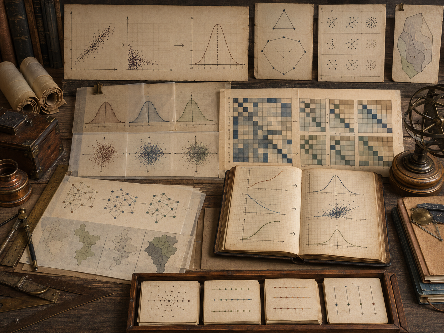
Linear algebra gives models a language of comparison. Vectors can be compared by length, direction, angle, distance, projection, similarity, rank, variance, or contribution to a transformation. Matrices can compare entities, variables, flows, features, states, sectors, documents, or network nodes.
But comparison is not automatic. If one column measures dollars in millions and another measures probability from zero to one, raw magnitudes can dominate computation. If one row represents a large region and another a small region, row totals can overwhelm proportional structure. If one vector is long because it is large rather than similar, Euclidean distance may answer the wrong question. Scaling and normalization decide what kind of comparison the model is allowed to make.
Why Scaling and Normalization Matter
Scaling and normalization matter because linear algebra computations are sensitive to magnitude, units, geometry, and numerical conditioning. A model may produce different distances, clusters, principal components, regressions, rankings, recommendations, or decompositions depending on whether values are raw, centered, standardized, normalized, logged, row-scaled, column-scaled, or transformed.
Scaling is not only a computational convenience. It changes the meaning of comparison. A raw-value model may compare absolute magnitude. A standardized model may compare relative position. A normalized-vector model may compare direction rather than size. A row-stochastic model may compare proportions or transition probabilities. These are different modeling claims.
| Scaling choice | What it emphasizes | What it may hide |
|---|---|---|
| Raw units | Absolute magnitude and original measurement meaning. | Variables with large units may dominate computation. |
| Centering | Deviation from a baseline or mean. | Absolute level may become less visible. |
| Standardization | Relative position measured in standard deviations. | Original units and real-world magnitude. |
| Min-max scaling | Relative location within an observed range. | Outlier influence and external comparability. |
| Vector normalization | Direction, profile, or pattern. | Total size or volume. |
| Row normalization | Composition, distribution, or probability. | Row totals and absolute scale. |
| Column normalization | Feature comparability across variables. | Original feature magnitude and domain units. |
The choice should follow the modeling question. Scaling without interpretation can make a model cleaner but less meaningful.
Comparative Structure Before Computation
Comparative structure is the model’s answer to the question: “Comparable in what sense?” Two cities may be comparable by population, energy use per capita, emissions intensity, infrastructure vulnerability, economic structure, or geographic exposure. Two documents may be comparable by word counts, normalized term frequencies, topic proportions, embeddings, or citation patterns.
\text{comparison} = \text{representation} + \text{scale} + \text{metric}
\]
Interpretation: Linear algebra comparison depends on how objects are represented, scaled, and measured geometrically.
A matrix does not define comparison by itself. The rows, columns, units, transformations, and metric determine whether the model compares size, shape, composition, distance, similarity, variance, dependence, transition, or influence.
| Comparison question | Possible scaling choice | Possible metric |
|---|---|---|
| Which entity is largest? | Raw units. | Magnitude, total, norm. |
| Which entity has a similar profile? | Row normalization or vector normalization. | Cosine similarity, correlation, angular distance. |
| Which variable varies most? | Centered data. | Variance, covariance, singular values. |
| Which variables are comparable despite units? | Standardization. | Euclidean distance, PCA on correlation structure. |
| Which state transition is probable? | Row-stochastic normalization. | Markov transition probability. |
| Which network node is influential? | Degree, row, column, or stochastic normalization. | Centrality, PageRank, spectral score. |
Scaling and normalization make comparison possible, but they also decide what comparison means.
Raw Units and Model Meaning
Raw units preserve original measurement meaning. If a column measures megawatts, dollars, tons, people, kilometers, or probabilities, raw units keep that meaning visible. This can be essential for policy interpretation, engineering constraints, physical conservation, accounting identities, budgets, and resource planning.
But raw units can distort computational comparison when variables have very different magnitudes. A feature measured in thousands may dominate a feature measured in decimals, even if the smaller-scale feature is substantively important.
| Raw-unit benefit | Raw-unit risk | Review question |
|---|---|---|
| Preserves physical or institutional meaning. | Large units can dominate distances and decompositions. | Is absolute magnitude the intended comparison? |
| Supports direct interpretation of coefficients. | Mixed units may weaken geometric comparison. | Can coefficients be compared across variables? |
| Protects accounting or conservation logic. | Numerical conditioning may suffer. | Does scaling preserve constraints? |
| Makes output legible to domain users. | Magnitude may hide pattern similarity. | Should the model compare size or profile? |
Raw units are often the right choice when the model’s purpose is absolute quantity. They are often risky when the purpose is geometric comparison across variables.
Centering and Standardization
Centering subtracts a reference value, usually the mean. Standardization subtracts the mean and divides by the standard deviation. These transformations shift interpretation from absolute value to relative deviation.
\tilde{x}_j = x_j-\mu_j
\qquad\qquad
z_j = \frac{x_j-\mu_j}{\sigma_j}
\]
Interpretation: Centering expresses values as deviations from a baseline; standardization expresses values as deviations measured in standard-deviation units.
Standardization is common before PCA, clustering, regression with regularization, nearest-neighbor models, and machine learning workflows. It can prevent high-magnitude variables from dominating. But it also changes interpretation: a one-unit change means one standard deviation, not one original unit.
| Transformation | Formula | Best suited for | Warning |
|---|---|---|---|
| Centering | \(x-\mu\) | Variance, covariance, PCA, deviations from baseline. | Absolute level is removed from the transformed values. |
| Standardization | \((x-\mu)/\sigma\) | Comparing variables with different units or variances. | Outliers can affect mean and standard deviation. |
| Robust scaling | Median and interquartile range. | Skewed distributions or outlier-sensitive data. | Interpretation shifts to robust relative position. |
| Group standardization | Within-group mean and standard deviation. | Comparisons within regions, cohorts, sectors, or periods. | Between-group absolute differences may be hidden. |
Standardization makes variables comparable by variation, not by original magnitude. That distinction should always be documented.
Min-Max Normalization and Range Scaling
Min-max normalization maps values into a chosen range, often from zero to one. It is useful when models require bounded inputs or when interpretation depends on relative position inside an observed range.
x’_j = \frac{x_j-\min(x_j)}{\max(x_j)-\min(x_j)}
\]
Interpretation: Min-max normalization expresses a value by its location within the observed minimum and maximum range.
Range scaling is easy to explain, but it can be sensitive to outliers and to changes in the dataset. A new extreme value can change all normalized values. It also depends on the observed sample, not necessarily on a meaningful external boundary.
| Use case | Benefit | Risk |
|---|---|---|
| Bounded model inputs | Places values in a predictable range. | Future values may fall outside the original range. |
| Index construction | Creates comparable indicators. | Indicator weights and ranges may embed judgment. |
| Visualization | Makes features visually comparable. | Can hide absolute magnitude and uncertainty. |
| Similarity workflows | Prevents large-scale features from dominating. | Outliers can compress most observations. |
Min-max normalization is useful when range comparison is the intended meaning. It is weaker when absolute scale, distribution shape, or out-of-sample stability matters.
Vector Normalization and Directional Comparison
Vector normalization rescales a vector to have length one. This preserves direction but removes magnitude. It is useful when the pattern or profile matters more than total size.
\hat{\mathbf{x}} = \frac{\mathbf{x}}{\|\mathbf{x}\|}
\]
Interpretation: Unit-vector normalization turns a vector into a direction, allowing comparison of profile rather than magnitude.
This is central to cosine similarity, document retrieval, embeddings, recommendation systems, directional comparison, and profile matching. Two vectors can point in similar directions even when one is much larger than the other.
| Comparison type | Vector normalization helps when | It is risky when |
|---|---|---|
| Document similarity | Text length should not dominate similarity. | Document size or intensity matters substantively. |
| Regional profiles | Composition matters more than total population. | Total need or capacity matters. |
| Embedding comparison | Direction encodes semantic similarity. | Embedding magnitude carries useful confidence or intensity. |
| Consumption patterns | Relative allocation matters. | Absolute consumption matters for policy or planning. |
Vector normalization answers a different question from raw magnitude comparison. It asks: “Are these vectors shaped similarly?” not “Are these vectors the same size?”
Row Normalization and Compositional Structure
Row normalization rescales each row, often so row entries sum to one or have unit norm. This is useful when rows represent distributions, profiles, probabilities, shares, or compositions.
p_{ij} = \frac{a_{ij}}{\sum_k a_{ik}}
\]
Interpretation: Row-sum normalization converts each row into a proportional profile.
Row normalization is common in Markov chains, input-output shares, document-term frequency profiles, transition matrices, household budget shares, sectoral composition, and network outflow proportions.
| Row-normalized structure | Meaning | Interpretive warning |
|---|---|---|
| Transition probabilities | Each row describes movement from one state to others. | External inflows or shocks may be omitted. |
| Budget shares | Each row describes allocation across categories. | Total budget size disappears. |
| Document-term frequencies | Each row describes term composition. | Document length becomes less visible. |
| Network outflow shares | Each row describes distribution of outgoing flow. | Total flow magnitude is removed. |
Row normalization is appropriate when composition matters more than total magnitude. It is inappropriate when total magnitude is central to the decision.
Column Normalization and Feature Comparability
Column normalization rescales variables or features so they can be compared or used together in a model without one column dominating because of unit scale. It is common before PCA, clustering, regression, optimization, and machine learning pipelines.
| Column operation | Effect | Use case |
|---|---|---|
| Mean centering | Columns become deviations from their means. | Covariance, PCA, regression diagnostics. |
| Unit variance scaling | Columns have comparable variance scale. | Correlation PCA, clustering, regularization. |
| Unit norm scaling | Columns have equal vector length. | Feature balancing, matrix factorization. |
| Max scaling | Columns are scaled by maximum magnitude. | Bounded feature comparison. |
| Domain scaling | Columns scaled by meaningful external constants. | Engineering, economics, public policy thresholds. |
Column normalization is not automatically neutral. Equalizing variables can be appropriate when features deserve equal computational weight. It can be inappropriate when real-world magnitude should determine influence.
Matrix Scaling and Conditioning
Scaling can improve numerical conditioning. Poorly scaled matrices can make solving systems, computing inverses, estimating ranks, or running iterative methods more fragile. Diagonal scaling attempts to balance rows or columns so computation becomes more stable.
\tilde{A}=D_r A D_c
\]
Interpretation: Row and column diagonal scaling can transform a matrix into a numerically better-balanced form.
Numerical scaling must be distinguished from interpretive scaling. A solver may benefit from a scaled matrix, but results may need to be transformed back into original units. Otherwise, computation may be stable while interpretation becomes confused.
| Scaling purpose | Computational benefit | Interpretive requirement |
|---|---|---|
| Row equilibration | Balances constraint magnitudes. | Track how constraints were rescaled. |
| Column equilibration | Balances variable magnitudes. | Transform solution units back when needed. |
| Preconditioning | Improves iterative solver convergence. | Document preconditioner and residual interpretation. |
| Nondimensionalization | Improves physical and numerical comparability. | Define characteristic scales and physical meaning. |
Scaling for numerical stability should be documented alongside scaling for model interpretation. They are related but not identical.
Normalization in Networks and Transition Models
Network matrices often need normalization. A binary adjacency matrix may become a degree-normalized matrix. A weighted matrix may become a transition matrix. A graph Laplacian may be normalized to compare nodes with different degrees. These transformations change the meaning of network structure.
P_{ij} = \frac{A_{ij}}{\sum_k A_{ik}}
\]
Interpretation: A row-normalized adjacency matrix becomes a transition matrix when row sums represent outgoing movement or probability.
| Network matrix | Normalization | Meaning |
|---|---|---|
| Adjacency matrix | None. | Raw connection or weight structure. |
| Row-stochastic matrix | Rows sum to one. | Outgoing transition probabilities or shares. |
| Column-stochastic matrix | Columns sum to one. | Incoming allocation or influence shares. |
| Normalized Laplacian | Degree-based normalization. | Connectivity adjusted for degree differences. |
| Flow-normalized matrix | Entries divided by total flow or capacity. | Relative flow intensity or utilization. |
Network normalization can reveal comparable structure across nodes. It can also erase the fact that some nodes carry much larger loads, risks, or responsibilities.
Scaling in PCA, SVD, and Embeddings
PCA and SVD are highly sensitive to scaling. PCA on raw covariance structure emphasizes variables with large variance. PCA on standardized variables emphasizes correlation structure. Both are valid, but they answer different questions.
X = U\Sigma V^T
\]
Interpretation: The singular vectors and singular values depend on how the data matrix \(X\) is centered, scaled, normalized, or transformed before decomposition.
Embeddings and dimensionality-reduction workflows also depend on scaling choices. Length normalization, centering, whitening, cosine similarity, and distance metrics can change neighborhoods, clusters, rankings, and retrieved results.
| Workflow | Scaling choice | Interpretation |
|---|---|---|
| PCA on covariance matrix | Centered raw variables. | Components emphasize high-variance variables. |
| PCA on correlation matrix | Standardized variables. | Components emphasize standardized relationships. |
| SVD of document-term matrix | Raw counts, TF, TF-IDF, or normalized rows. | Latent structure depends on text representation. |
| Embedding similarity | Raw vectors or unit vectors. | Comparison may emphasize magnitude or direction. |
| Whitening | Decorrelated and variance-normalized components. | Improves some algorithms but changes geometry. |
Scaling choices should be reported whenever PCA, SVD, embeddings, clustering, or similarity results are interpreted.
Distance, Similarity, and Geometry
Scaling and normalization shape geometry. Euclidean distance, cosine similarity, dot products, projections, norms, covariance, correlation, and nearest neighbors all depend on the representation and scale of the vectors being compared.
\cos(\theta)=\frac{\mathbf{x}\cdot\mathbf{y}}{\|\mathbf{x}\|\,\|\mathbf{y}\|}
\]
Interpretation: Cosine similarity compares direction rather than raw magnitude.
| Geometry choice | Emphasizes | Scaling concern |
|---|---|---|
| Euclidean distance | Absolute coordinate differences. | Large-scale variables dominate unless scaled. |
| Cosine similarity | Directional similarity. | Magnitude information is removed. |
| Correlation | Centered co-variation. | Mean and scale are removed. |
| Dot product | Alignment weighted by magnitude. | Large vectors produce larger scores. |
| Mahalanobis distance | Distance adjusted by covariance structure. | Requires reliable covariance estimation. |
The metric should match the modeling purpose. Geometry is not only mathematical; it defines the meaning of closeness, similarity, separation, and influence.
Scale Sensitivity and Interpretation
Scale sensitivity asks whether conclusions change under different reasonable scaling choices. This is a form of representation sensitivity. A result that appears under raw units but disappears after standardization may depend on magnitude. A result that appears only after normalization may depend on relative profile rather than size.
X_{\text{raw}},\; X_{\text{centered}},\; X_{\text{standardized}},\; X_{\text{normalized}}
\longrightarrow
\text{compare conclusions}
\]
Interpretation: Comparing outputs across scaling choices helps identify which conclusions depend on the chosen scale.
| Scale-sensitive result | Possible meaning | Responsible response |
|---|---|---|
| Cluster changes after standardization. | Clusters depended on high-magnitude variables. | Explain whether size or profile should drive grouping. |
| PCA components change after scaling. | Variance structure depended on units. | Report whether PCA used covariance or correlation structure. |
| Nearest neighbors change after normalization. | Similarity depended on direction rather than magnitude. | Clarify whether pattern or size is the modeling target. |
| Solver improves after scaling. | Numerical conditioning was affected by units. | Report scaling and back-transform interpretation. |
| Ranking changes after row normalization. | Total size was removed from comparison. | State whether totals or proportions matter. |
Scale-sensitive conclusions are not automatically wrong. They require careful interpretation because they depend on what kind of comparison the model was designed to make.
Mathematical Deepening
This section adds a more formal layer. Scaling and normalization connect units, vector norms, matrix norms, diagonal transformations, conditioning, covariance, correlation, row-stochastic matrices, unit-vector geometry, PCA, SVD, embeddings, distance metrics, similarity metrics, and responsible interpretation.
Scale Design Review
Comparison Target
State whether the workflow compares absolute magnitude, relative deviation, distribution, direction, probability, or profile.
Unit Meaning
Document original units before any transformation is applied.
Transformation Rule
Record centering, standardization, normalization, log scaling, row scaling, or column scaling formulas.
Back-Transformation
When needed, explain how scaled outputs map back to original units.
Comparative Geometry Review
Norm Choice
Specify whether vector length, matrix norm, row norm, column norm, or weighted norm drives comparison.
Metric Choice
Explain whether distance, angle, correlation, dot product, projection, or covariance defines similarity.
Direction vs Magnitude
Clarify whether normalized vectors are being compared by profile rather than total size.
Distribution vs Total
State whether row normalization removes meaningful total volume.
Numerical Review
Conditioning
Check whether scaling improves or worsens condition numbers, residuals, and solver behavior.
Diagonal Scaling
Document row and column scaling matrices when they are used for numerical balancing.
Outliers
Review how outliers affect means, standard deviations, ranges, and scaled values.
Stability
Compare results under reasonable alternative scaling choices.
Governance Review
Scaling Register
Maintain a structured record of transformation choices, formulas, purposes, and interpretation warnings.
Sensitivity Comparison
Compare conclusions across raw, centered, standardized, normalized, and domain-scaled representations.
Documentation
Preserve scale choices in notebooks, schemas, metadata, README files, and generated reports.
Responsible Use
Communicate whether outputs represent magnitude, relative position, profile, direction, or probability.
Examples from Systems Modeling
Scaling and normalization appear wherever systems are compared through matrices, vectors, features, networks, state spaces, or embeddings.
Infrastructure Risk
Demand, outage exposure, repair cost, population served, and network centrality may have different units. Scaling determines whether the model prioritizes size, vulnerability, or relative risk.
Economic Input-Output Models
Raw flows preserve economic magnitude, while normalized technical coefficients reveal sector dependence and proportional production structure.
Machine Learning Pipelines
Feature standardization can determine which variables dominate distance, regularization, PCA, clustering, and classifier behavior.
Climate and Energy Systems
Temperature, demand, emissions, generation, storage, and cost variables require careful scaling before joint analysis or dimensionality reduction.
Public Health Models
Counts, rates, probabilities, demographic shares, and regional totals require different normalization choices depending on whether burden or risk is being compared.
Knowledge Retrieval
Document length, term frequency, TF-IDF weighting, embedding normalization, and cosine similarity define what counts as textual or semantic closeness.
Across these examples, scaling choices decide whether the model compares totals, proportions, deviations, directions, probabilities, or patterns.
Computation and Reproducible Workflows
Computational workflows for scaling, normalization, and comparative structure should document original units, scale ranges, means, standard deviations, row sums, column norms, missing-value rules, outlier treatment, transformation formulas, scaling purpose, back-transformation rules, distance metrics, similarity metrics, conditioning changes, sensitivity comparisons, validation checks, and interpretation warnings.
The companion repository treats scaling as an auditable modeling layer. Python, R, Julia, SQL, Haskell, C, C++, Fortran, Rust, Go, notebooks, schemas, generated outputs, Canvas artifacts, advanced reports, and calculators each support a different layer of scaling diagnostics, normalization comparison, sensitivity review, and responsible interpretation.
For this article, the computational examples compare raw, centered, standardized, min-max normalized, row-normalized, and vector-normalized representations for a small systems matrix. The workflow records how transformation choices change norms, column comparability, row profiles, and interpretation.
Python Workflow: Scaling and Normalization Audit
The Python workflow below creates a compact scaling audit. It compares raw values, standardized columns, min-max scaled columns, row-sum normalized rows, and unit-vector normalized rows, then exports diagnostic records and interpretation warnings.
from __future__ import annotations

from dataclasses import asdict, dataclass
from pathlib import Path
import csv
import json
import math


@dataclass(frozen=True)
class ScalingNormalizationAudit:
    workflow_name: str
    matrix_shape: str
    row_meaning: str
    column_meaning: str
    raw_column_norm_1: float
    raw_column_norm_2: float
    standardized_column_norm_1: float
    standardized_column_norm_2: float
    minmax_column_min_1: float
    minmax_column_max_1: float
    first_row_sum_after_row_normalization: float
    first_row_norm_after_unit_normalization: float
    raw_condition_proxy: float
    standardized_condition_proxy: float
    comparison_warning: str
    interpretation_warning: str


def column(A: list[list[float]], j: int) -> list[float]:
    return [row[j] for row in A]


def mean(values: list[float]) -> float:
    return sum(values) / len(values)


def std(values: list[float]) -> float:
    m = mean(values)
    return math.sqrt(sum((x - m) ** 2 for x in values) / len(values))


def norm2(values: list[float]) -> float:
    return math.sqrt(sum(x * x for x in values))


def transpose(A: list[list[float]]) -> list[list[float]]:
    return [list(col) for col in zip(*A)]


def standardize_columns(A: list[list[float]]) -> list[list[float]]:
    cols = transpose(A)
    means = [mean(col) for col in cols]
    stds = [std(col) or 1.0 for col in cols]
    return [[(row[j] - means[j]) / stds[j] for j in range(len(row))] for row in A]


def minmax_columns(A: list[list[float]]) -> list[list[float]]:
    cols = transpose(A)
    mins = [min(col) for col in cols]
    maxs = [max(col) for col in cols]
    ranges = [(maxs[j] - mins[j]) or 1.0 for j in range(len(cols))]
    return [[(row[j] - mins[j]) / ranges[j] for j in range(len(row))] for row in A]


def row_sum_normalize(A: list[list[float]]) -> list[list[float]]:
    normalized = []
    for row in A:
        total = sum(row) or 1.0
        normalized.append([x / total for x in row])
    return normalized


def unit_row_normalize(A: list[list[float]]) -> list[list[float]]:
    normalized = []
    for row in A:
        length = norm2(row) or 1.0
        normalized.append([x / length for x in row])
    return normalized


def frobenius_norm(A: list[list[float]]) -> float:
    return math.sqrt(sum(value * value for row in A for value in row))


def condition_proxy(A: list[list[float]]) -> float:
    # Portable proxy for scale imbalance in a small teaching matrix.
    column_norms = [norm2(column(A, j)) for j in range(len(A[0]))]
    return max(column_norms) / max(min(column_norms), 1e-15)


def build_audit() -> ScalingNormalizationAudit:
    # Rows represent infrastructure zones.
    # Columns represent annual demand and outage exposure in very different units.
    A_raw = [
        [1200.0, 0.08],
        [1800.0, 0.15],
        [900.0, 0.04],
    ]

    A_standardized = standardize_columns(A_raw)
    A_minmax = minmax_columns(A_raw)
    A_row_sum = row_sum_normalize(A_raw)
    A_unit_rows = unit_row_normalize(A_raw)

    return ScalingNormalizationAudit(
        workflow_name="scaling_normalization_audit",
        matrix_shape="3x2",
        row_meaning="infrastructure_zones",
        column_meaning="annual_demand_and_outage_exposure",
        raw_column_norm_1=round(norm2(column(A_raw, 0)), 12),
        raw_column_norm_2=round(norm2(column(A_raw, 1)), 12),
        standardized_column_norm_1=round(norm2(column(A_standardized, 0)), 12),
        standardized_column_norm_2=round(norm2(column(A_standardized, 1)), 12),
        minmax_column_min_1=round(min(column(A_minmax, 0)), 12),
        minmax_column_max_1=round(max(column(A_minmax, 0)), 12),
        first_row_sum_after_row_normalization=round(sum(A_row_sum[0]), 12),
        first_row_norm_after_unit_normalization=round(norm2(A_unit_rows[0]), 12),
        raw_condition_proxy=round(condition_proxy(A_raw), 12),
        standardized_condition_proxy=round(condition_proxy(A_standardized), 12),
        comparison_warning=(
            "Raw units compare magnitude; standardized columns compare relative position; "
            "row normalization compares composition; unit-vector normalization compares direction."
        ),
        interpretation_warning=(
            "Scaling and normalization change what comparison means. "
            "Every transformed matrix should record original units, transformation rule, purpose, and interpretation limits."
        ),
    )


def write_outputs(output_dir: Path) -> None:
    (output_dir / "tables").mkdir(parents=True, exist_ok=True)
    (output_dir / "json").mkdir(parents=True, exist_ok=True)
    (output_dir / "reports").mkdir(parents=True, exist_ok=True)

    audit = build_audit()
    row = asdict(audit)

    with (output_dir / "tables" / "scaling_normalization_audit.csv").open(
        "w", newline="", encoding="utf-8"
    ) as handle:
        writer = csv.DictWriter(handle, fieldnames=list(row.keys()))
        writer.writeheader()
        writer.writerow(row)

    (output_dir / "json" / "scaling_normalization_audit.json").write_text(
        json.dumps(row, indent=2, sort_keys=True),
        encoding="utf-8",
    )

    report = [
        "# Scaling and Normalization Audit",
        "",
        f"- Workflow: {audit.workflow_name}",
        f"- Matrix shape: {audit.matrix_shape}",
        f"- Raw column norm 1: {audit.raw_column_norm_1}",
        f"- Raw column norm 2: {audit.raw_column_norm_2}",
        f"- Standardized column norm 1: {audit.standardized_column_norm_1}",
        f"- Standardized column norm 2: {audit.standardized_column_norm_2}",
        f"- Raw condition proxy: {audit.raw_condition_proxy}",
        f"- Standardized condition proxy: {audit.standardized_condition_proxy}",
        "",
        audit.comparison_warning,
        "",
        audit.interpretation_warning,
    ]

    (output_dir / "reports" / "scaling_normalization_audit.md").write_text(
        "\\n".join(report) + "\\n",
        encoding="utf-8",
    )


if __name__ == "__main__":
    write_outputs(Path("outputs"))
    print("Scaling and normalization audit complete.")
This workflow makes scaling choices visible as model assumptions rather than hidden preprocessing steps.
R Workflow: Comparative Scaling Diagnostics
R can support the same audit by comparing raw, standardized, min-max, row-normalized, and unit-row-normalized representations.
A_raw <- matrix(
  c(
    1200.0, 0.08,
    1800.0, 0.15,
    900.0, 0.04
  ),
  nrow = 3,
  byrow = TRUE
)

colnames(A_raw) <- c("annual_demand", "outage_exposure")
rownames(A_raw) <- c("zone_a", "zone_b", "zone_c")

norm2 <- function(x) sqrt(sum(x^2))

minmax_columns <- function(A) {
  apply(A, 2, function(col) {
    rng <- max(col) - min(col)
    if (rng == 0) rep(0, length(col)) else (col - min(col)) / rng
  })
}

row_sum_normalize <- function(A) {
  totals <- rowSums(A)
  totals[totals == 0] <- 1
  A / totals
}

unit_row_normalize <- function(A) {
  norms <- apply(A, 1, norm2)
  norms[norms == 0] <- 1
  A / norms
}

condition_proxy <- function(A) {
  column_norms <- apply(A, 2, norm2)
  max(column_norms) / max(min(column_norms), 1e-15)
}

A_standardized <- scale(A_raw)
A_minmax <- minmax_columns(A_raw)
A_row_sum <- row_sum_normalize(A_raw)
A_unit_rows <- unit_row_normalize(A_raw)

audit_record <- data.frame(
  workflow_name = "scaling_normalization_audit",
  matrix_shape = paste(dim(A_raw), collapse = "x"),
  row_meaning = "infrastructure_zones",
  column_meaning = "annual_demand_and_outage_exposure",
  raw_column_norm_1 = norm2(A_raw[, 1]),
  raw_column_norm_2 = norm2(A_raw[, 2]),
  standardized_column_norm_1 = norm2(A_standardized[, 1]),
  standardized_column_norm_2 = norm2(A_standardized[, 2]),
  minmax_column_min_1 = min(A_minmax[, 1]),
  minmax_column_max_1 = max(A_minmax[, 1]),
  first_row_sum_after_row_normalization = sum(A_row_sum[1, ]),
  first_row_norm_after_unit_normalization = norm2(A_unit_rows[1, ]),
  raw_condition_proxy = condition_proxy(A_raw),
  standardized_condition_proxy = condition_proxy(A_standardized),
  comparison_warning = paste(
    "Raw units compare magnitude; standardized columns compare relative position;",
    "row normalization compares composition; unit-vector normalization compares direction."
  ),
  interpretation_warning = paste(
    "Scaling and normalization change what comparison means.",
    "Every transformed matrix should record original units, transformation rule,",
    "purpose, and interpretation limits."
  )
)

dir.create("outputs/tables", recursive = TRUE, showWarnings = FALSE)
write.csv(
  audit_record,
  "outputs/tables/r_scaling_normalization_audit.csv",
  row.names = FALSE
)

print(audit_record)
This R workflow makes scale imbalance, standardized comparability, row profiles, and interpretation warnings explicit.
Haskell Workflow: Typed Scaling Records
Haskell can represent scaling and normalization decisions as typed records, keeping transformation rules and interpretation warnings attached to the workflow output.
module Main where

data ScalingNormalizationAudit = ScalingNormalizationAudit
  { workflowName :: String
  , matrixShape :: String
  , rowMeaning :: String
  , columnMeaning :: String
  , rawColumnNorm1 :: Double
  , rawColumnNorm2 :: Double
  , standardizedColumnNorm1 :: Double
  , standardizedColumnNorm2 :: Double
  , rawConditionProxy :: Double
  , standardizedConditionProxy :: Double
  , comparisonWarning :: String
  , interpretationWarning :: String
  } deriving (Show)

buildAudit :: ScalingNormalizationAudit
buildAudit =
  ScalingNormalizationAudit
    "scaling_normalization_audit"
    "3x2"
    "infrastructure_zones"
    "annual_demand_and_outage_exposure"
    2345.21
    0.1749
    1.4142
    1.4142
    13406.31
    1.0
    "Raw units compare magnitude; standardized columns compare relative position; row normalization compares composition; unit-vector normalization compares direction."
    "Scaling and normalization change what comparison means. Every transformed matrix should record original units, transformation rule, purpose, and interpretation limits."

main :: IO ()
main =
  print buildAudit
The typed record keeps scale choice, comparative purpose, and interpretive warning together.
SQL Workflow: Scaling Governance Registry
SQL can document scaling assumptions when matrix workflows support reports, dashboards, repositories, audits, or institutional decision systems.
CREATE TABLE scaling_governance_registry (
    assumption_key TEXT PRIMARY KEY,
    assumption_name TEXT NOT NULL,
    modeling_role TEXT NOT NULL,
    transformation_role TEXT NOT NULL,
    review_warning TEXT NOT NULL
);

INSERT INTO scaling_governance_registry VALUES
(
  'raw_units',
  'Raw units',
  'Preserves original measurement meaning.',
  'Keeps values in domain units such as dollars, tons, kilometers, rates, or probabilities.',
  'Raw magnitudes can dominate computation when units differ widely.'
);

INSERT INTO scaling_governance_registry VALUES
(
  'centering',
  'Centering',
  'Represents values as deviations from a baseline.',
  'Subtracts means or reference values before variance, covariance, PCA, or regression analysis.',
  'Centering removes absolute level from the transformed representation.'
);

INSERT INTO scaling_governance_registry VALUES
(
  'standardization',
  'Standardization',
  'Makes variables comparable by relative variation.',
  'Subtracts mean and divides by standard deviation.',
  'Standardization changes interpretation from original units to standard-deviation units.'
);

INSERT INTO scaling_governance_registry VALUES
(
  'minmax_normalization',
  'Min-max normalization',
  'Represents values by location within an observed range.',
  'Maps values to a bounded interval such as zero to one.',
  'Outliers and changing ranges can shift normalized values.'
);

INSERT INTO scaling_governance_registry VALUES
(
  'vector_normalization',
  'Vector normalization',
  'Compares direction or profile rather than magnitude.',
  'Divides vectors by their norms.',
  'Total size is removed from the comparison.'
);

INSERT INTO scaling_governance_registry VALUES
(
  'row_normalization',
  'Row normalization',
  'Represents each row as a distribution, share, or probability profile.',
  'Divides row entries by row totals or row norms.',
  'Row totals disappear unless preserved separately.'
);

INSERT INTO scaling_governance_registry VALUES
(
  'column_normalization',
  'Column normalization',
  'Balances feature influence across columns.',
  'Scales columns by variance, norm, range, or domain constant.',
  'Feature magnitudes may no longer reflect real-world size.'
);

INSERT INTO scaling_governance_registry VALUES
(
  'condition_scaling',
  'Conditioning-oriented scaling',
  'Improves numerical balance and solver behavior.',
  'Uses diagonal scaling, equilibration, nondimensionalization, or preconditioning.',
  'Scaled numerical results must be interpreted or transformed back carefully.'
);

INSERT INTO scaling_governance_registry VALUES
(
  'scale_sensitivity',
  'Scale sensitivity',
  'Tests whether conclusions depend on scaling choices.',
  'Compares outputs across raw, centered, standardized, normalized, and domain-scaled matrices.',
  'Scale-sensitive conclusions require explicit interpretation warnings.'
);

SELECT
    assumption_name,
    modeling_role,
    transformation_role,
    review_warning
FROM scaling_governance_registry
ORDER BY assumption_key;
This registry keeps scaling choices tied to raw units, centering, standardization, normalization, conditioning, sensitivity, and responsible interpretation.
GitHub Repository
The companion repository for this article is designed as a reproducible mathematical-modeling workspace. It supports scaling audits, normalization comparisons, matrix transformation records, column-norm diagnostics, row-profile checks, condition proxies, governance tables, generated artifacts, advanced mathematical audit reports, and reusable calculator scripts.
Complete Code Repository
Companion article folder with Python, R, Julia, SQL, Haskell, C, C++, Fortran, Rust, Go, notebooks, documentation, synthetic teaching data, generated outputs, schemas, Canvas-ready workflow artifacts, and reusable calculator scripts for scaling, normalization, comparative structure, raw units, centering, standardization, min-max normalization, vector normalization, row normalization, column normalization, matrix scaling, conditioning, network normalization, PCA, SVD, embeddings, distance metrics, similarity metrics, scale sensitivity, governance, and responsible systems modeling.
Interpretive Limits and Responsible Use
Scaling and normalization are powerful because they make comparison possible. They can prevent large units from dominating, improve numerical stability, clarify relative structure, support probability interpretation, reveal profile similarity, and make high-dimensional workflows more coherent.
Their limits are equally important. Scaling can remove absolute magnitude. Normalization can erase totals. Standardization can hide real-world units. Min-max scaling can depend on observed extremes. Vector normalization can treat small and large entities as directionally equivalent. Row normalization can turn resource burden into proportional profile. A model can become more computationally balanced while becoming less substantively transparent.
Responsible use requires documenting original units, transformation formulas, scaling purpose, comparison metric, numerical effects, outlier sensitivity, back-transformation rules, validation evidence, and interpretation boundaries. Scaling choices should be treated as modeling assumptions because they define what kind of comparison the linear algebra model is allowed to make.
Related Articles
- What Is Linear Algebra for Systems Modeling?
- Representation Choices and Model Assumptions
- When Linear Models Clarify and When They Distort
- Interpretation, Approximation, and Responsible Mathematical Modeling
- Matrix Operations Across Modeling Languages
- Visualization of Vectors, Transformations, and State Spaces
- Numerical Stability and Conditioning
- Decomposition Workflows for Systems Analysis
- Scientific Computing Workflows for Linear Algebra
- Reproducible Linear Algebra Workflows with Notebooks and Documentation
- Singular Value Decomposition
- Principal Component Analysis
- Dimensionality Reduction Techniques
- Machine Learning and Linear Algebra
- Network Adjacency Matrices
- Linear Algebra for Systems Modeling
- Mathematical Modeling
- Systems Modeling
Further Reading
- Demmel, J.W. (1997) Applied Numerical Linear Algebra. Philadelphia, PA: SIAM. Available at: https://epubs.siam.org/doi/book/10.1137/1.9781611971446.
- Golub, G.H. and Van Loan, C.F. (2013) Matrix Computations. 4th edn. Baltimore, MD: Johns Hopkins University Press. Available at: https://jhupbooks.press.jhu.edu/title/matrix-computations.
- Higham, N.J. (2002) Accuracy and Stability of Numerical Algorithms. 2nd edn. Philadelphia, PA: SIAM. Available at: https://epubs.siam.org/doi/book/10.1137/1.9780898718027.
- Hastie, T., Tibshirani, R. and Friedman, J. (2009) The Elements of Statistical Learning. 2nd edn. New York: Springer. Available at: https://hastie.su.domains/ElemStatLearn/.
- Jolliffe, I.T. and Cadima, J. (2016) ‘Principal component analysis: a review and recent developments’, Philosophical Transactions of the Royal Society A, 374(2065), 20150202. Available at: https://doi.org/10.1098/rsta.2015.0202.
- Saad, Y. (2003) Iterative Methods for Sparse Linear Systems. 2nd edn. Philadelphia, PA: SIAM. Available at: https://www-users.cse.umn.edu/~saad/books.html.
- Saltelli, A. et al. (2008) Global Sensitivity Analysis: The Primer. Chichester: Wiley. Available at: https://doi.org/10.1002/9780470725184.
- Strang, G. (2019) Linear Algebra and Learning from Data. Wellesley, MA: Wellesley-Cambridge Press. Available at: https://math.mit.edu/~gs/learningfromdata/.
- Trefethen, L.N. and Bau, D. (1997) Numerical Linear Algebra. Philadelphia, PA: SIAM. Available at: https://epubs.siam.org/doi/book/10.1137/1.9780898719574.
- Wilkinson, J.H. (1965) The Algebraic Eigenvalue Problem. Oxford: Clarendon Press. Available at: https://global.oup.com/academic/product/the-algebraic-eigenvalue-problem-9780198534181.
References
- Demmel, J.W. (1997) Applied Numerical Linear Algebra. Philadelphia, PA: SIAM. Available at: https://epubs.siam.org/doi/book/10.1137/1.9781611971446.
- Golub, G.H. and Van Loan, C.F. (2013) Matrix Computations. 4th edn. Baltimore, MD: Johns Hopkins University Press. Available at: https://jhupbooks.press.jhu.edu/title/matrix-computations.
- Higham, N.J. (2002) Accuracy and Stability of Numerical Algorithms. 2nd edn. Philadelphia, PA: SIAM. Available at: https://epubs.siam.org/doi/book/10.1137/1.9780898718027.
- Hastie, T., Tibshirani, R. and Friedman, J. (2009) The Elements of Statistical Learning. 2nd edn. New York: Springer. Available at: https://hastie.su.domains/ElemStatLearn/.
- Jolliffe, I.T. and Cadima, J. (2016) ‘Principal component analysis: a review and recent developments’, Philosophical Transactions of the Royal Society A, 374(2065), 20150202. Available at: https://doi.org/10.1098/rsta.2015.0202.
- Saad, Y. (2003) Iterative Methods for Sparse Linear Systems. 2nd edn. Philadelphia, PA: SIAM. Available at: https://www-users.cse.umn.edu/~saad/books.html.
- Saltelli, A. et al. (2008) Global Sensitivity Analysis: The Primer. Chichester: Wiley. Available at: https://doi.org/10.1002/9780470725184.
- Strang, G. (2019) Linear Algebra and Learning from Data. Wellesley, MA: Wellesley-Cambridge Press. Available at: https://math.mit.edu/~gs/learningfromdata/.
- Trefethen, L.N. and Bau, D. (1997) Numerical Linear Algebra. Philadelphia, PA: SIAM. Available at: https://epubs.siam.org/doi/book/10.1137/1.9780898719574.
- Wilkinson, J.H. (1965) The Algebraic Eigenvalue Problem. Oxford: Clarendon Press. Available at: https://global.oup.com/academic/product/the-algebraic-eigenvalue-problem-9780198534181.