
Last Updated July 4, 2026
Visualization of vectors, transformations, and state spaces explains how linear algebra becomes visible: as direction, magnitude, rotation, scaling, projection, subspace structure, trajectories, uncertainty, and system behavior. In systems modeling, visualization is not decoration. It is a way to inspect mathematical structure, diagnose computation, communicate assumptions, and interpret how variables move together.
This article continues Part VIII of the Linear Algebra for Systems Modeling series by connecting vectors, coordinate systems, bases, matrices, transformations, projections, eigenvectors, eigenspaces, subspaces, null spaces, column spaces, rank, state spaces, phase portraits, trajectories, vector fields, PCA, SVD, dimensionality reduction, sparse networks, residual plots, uncertainty bands, and responsible visual interpretation.
The central modeling question is not only “Can this vector or matrix be plotted?” It is “What mathematical structure does the visualization reveal, what does it hide, and how should the visual evidence be interpreted in relation to the system being modeled?”
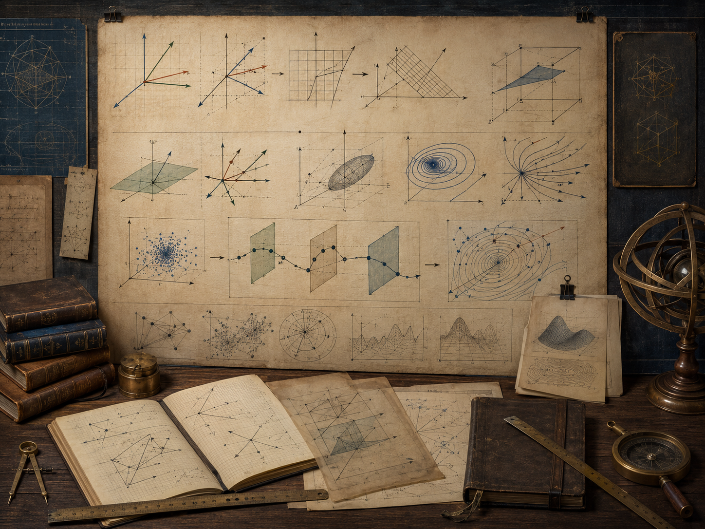
Linear algebra is often introduced symbolically, but many of its most important ideas are geometric. A vector has direction and magnitude. A matrix transforms space. A basis defines coordinates. A projection separates signal from residual. An eigenvector reveals a direction preserved by transformation. A trajectory shows how a state evolves through time. A cloud of points can reveal clustering, correlation, dimensional structure, or model failure.
Visualization helps make those structures inspectable. It can show whether variables are aligned, whether a transformation stretches or rotates a space, whether a system converges or diverges, whether a model has low-dimensional structure, whether residuals have pattern, whether uncertainty is concentrated, and whether an algorithm has produced a result that deserves interpretation.
Why Visualization Matters
Visualization matters because linear algebra often describes structure that is easier to understand geometrically than symbolically. A matrix equation can be correct and still obscure what is happening. A visualization can reveal alignment, distortion, collapse, rotation, separation, instability, clustering, or residual structure that a table of numbers may hide.
In systems modeling, visualization supports three kinds of work. First, it helps explain mathematical structure. Second, it helps diagnose numerical and modeling problems. Third, it helps communicate uncertainty and interpretation limits. A good visualization does not replace mathematics. It makes the mathematics inspectable.
| Visualization purpose | Linear algebra object | Modeling question |
|---|---|---|
| Geometric explanation | Vectors, bases, transformations. | What structure does the matrix or vector represent? |
| Numerical diagnosis | Residuals, ranks, singular values, condition numbers. | Is the computation reliable enough to interpret? |
| System behavior | State trajectories and vector fields. | How does the system move through time or state space? |
| Dimensional structure | PCA, SVD, embeddings, projections. | Can high-dimensional behavior be summarized responsibly? |
| Network structure | Adjacency, incidence, Laplacian matrices. | Which relationships shape flow, influence, or vulnerability? |
| Communication | Plots, maps, dashboards, reports. | What does the viewer need to know, and what could be misleading? |
Visual evidence should always be tied back to mathematical definitions, data construction, and model assumptions.
Vectors as Direction and Magnitude
A vector can represent a point, a displacement, a direction, a state, a feature profile, a force, a flow, a gradient, or a change in system variables. In two or three dimensions, vectors can be drawn directly as arrows. In higher dimensions, they must be summarized through projections, components, norms, similarity, or dimensionality reduction.
\mathbf{v}=
\begin{bmatrix}
v_1\\
v_2\\
\vdots\\
v_n
\end{bmatrix}
\]
Interpretation: A vector stores ordered components that can represent direction, magnitude, state, or measured attributes.
The norm of a vector gives a measure of magnitude:
\|\mathbf{v}\|_2=\sqrt{v_1^2+v_2^2+\cdots+v_n^2}
\]
Interpretation: The Euclidean norm measures the length of a vector in coordinate space.
| Vector visualization | What it shows | Systems modeling use |
|---|---|---|
| Arrow plot | Direction and magnitude. | Forces, gradients, flows, displacement, change. |
| Component bar | Contribution of each coordinate. | Feature profiles, sector weights, state composition. |
| Angle plot | Similarity or alignment. | Vector similarity, policy alignment, feature correlation. |
| Norm comparison | Relative magnitude. | Residual size, state magnitude, shock intensity. |
| Projection plot | Part of one vector explained by another direction. | Signal extraction, regression geometry, dimensional reduction. |
Vector visualization should make clear whether the vector represents a point, a direction, a state, a change, or a measurement profile. Those meanings are not interchangeable.
Coordinates, Bases, and Reference Frames
Coordinates depend on a basis. A vector can have different coordinate descriptions under different basis choices while representing the same geometric object. This matters in modeling because variables, units, coordinate systems, principal components, eigenvectors, and latent factors all define reference frames.
\mathbf{x}=c_1\mathbf{b}_1+c_2\mathbf{b}_2+\cdots+c_n\mathbf{b}_n
\]
Interpretation: A vector is represented as a combination of basis vectors.
Changing a basis can make structure easier to see. PCA rotates a coordinate system toward directions of high variance. Eigenvector coordinates can reveal stable modes. Orthogonal bases can separate independent components. But basis changes can also obscure the original variables that carried real-world meaning.
| Reference frame | Visual meaning | Interpretive risk |
|---|---|---|
| Original variables | Coordinates match measured quantities. | Correlated variables may hide structure. |
| Scaled variables | Coordinates adjust for units and magnitude. | Scaling choices can change visual emphasis. |
| Principal components | Axes follow dominant variance directions. | Components may be harder to interpret substantively. |
| Eigenbasis | Axes follow transformation-preserved directions. | Useful only when eigenstructure is meaningful and stable. |
| Latent factors | Axes summarize hidden structure. | Factors can be overinterpreted as real entities. |
A visualization should disclose the coordinate frame. Without that, the viewer may mistake a modeling representation for the underlying system itself.
Matrices as Transformations
A matrix can be visualized as a transformation of space. It may rotate, stretch, shear, compress, reflect, project, or collapse vectors. The matrix-vector product expresses this action:
\mathbf{y}=A\mathbf{x}
\]
Interpretation: The matrix \(A\) transforms an input vector \(\mathbf{x}\) into an output vector \(\mathbf{y}\).
One effective visualization is a transformed grid. A regular coordinate grid is shown before and after applying a matrix. If the grid rotates, stretches, shears, or collapses, the transformation becomes visible.
| Transformation | Visual sign | Modeling interpretation |
|---|---|---|
| Scaling | Grid expands or contracts along directions. | Variables are amplified or dampened. |
| Rotation | Axes turn without changing lengths equally. | Coordinate relationships are reoriented. |
| Shear | Right angles become slanted. | Variables influence each other asymmetrically. |
| Projection | Space collapses onto a line or plane. | Information is reduced to a lower-dimensional structure. |
| Reflection | Orientation flips across an axis or plane. | Signs or directions are reversed. |
| Near-singular collapse | Area or volume almost disappears. | Information loss or instability may be present. |
Visualizing a matrix as a transformation helps connect computation to system interpretation. It shows what the matrix does, not only what numbers it contains.
Matrix Multiplication as Composition
Matrix multiplication can be visualized as applying one transformation after another:
C=AB
\]
Interpretation: The product \(AB\) represents a composed transformation: first one transformation, then another, depending on convention and vector orientation.
Composition matters in modeling because workflows often chain transformations: scaling, centering, projection, rotation, feature extraction, filtering, simulation update, and prediction. Visualizing the chain can reveal where distortion, compression, or instability enters.
| Composition example | Matrix interpretation | Visual diagnostic |
|---|---|---|
| Scaling then rotation | Variables are normalized before coordinate reorientation. | Check whether scaling changes visual relationships. |
| Projection then regression | Data are reduced before model fitting. | Check what information is discarded. |
| Transition repeated over time | State evolves by repeated matrix application. | Check convergence, cycling, or divergence. |
| Feature transform then classifier | Input space is transformed before decision boundary. | Check whether separation is stable. |
| Network diffusion | State propagates through adjacency or transition structure. | Check where influence concentrates. |
Visualizing composed transformations can prevent a pipeline from becoming a black box of matrix operations.
Projections and Decompositions
Projection separates a vector into a component along a chosen subspace and a residual component outside that subspace. In regression, dimensionality reduction, signal extraction, and approximation, projection is one of the most important visual ideas in linear algebra.
\mathbf{x}=\hat{\mathbf{x}}+\mathbf{r}
\]
Interpretation: A vector can be decomposed into an approximated component \(\hat{\mathbf{x}}\) and a residual component \(\mathbf{r}\).
Decomposition visualizations show what part of the data is explained by a subspace and what remains. QR decomposition, SVD, PCA, least squares, and orthogonal projection all benefit from visual explanation when dimensions permit.
| Visualization | Linear algebra idea | Modeling use |
|---|---|---|
| Projection onto a line | Component along a direction. | Signal extraction and one-factor approximation. |
| Projection onto a plane | Approximation by a subspace. | Least squares and dimensional reduction. |
| Residual arrow | Unexplained component. | Model error and diagnostic review. |
| Orthogonal basis plot | Independent coordinate directions. | QR, PCA, and interpretable decomposition. |
| Singular value plot | Energy or variance by component. | Rank selection and compression review. |
A projection visualization should show both what is retained and what is lost. The residual is not an afterthought; it is part of the model evidence.
Subspaces, Rank, and Null Structure
Subspaces are central to linear algebra. The column space shows what outputs a matrix can produce. The null space shows what inputs the matrix collapses to zero. Rank shows the dimension of independent output structure.
A\mathbf{x}=\mathbf{0}
\]
Interpretation: The null space contains inputs that disappear under the matrix transformation.
Visualizing subspaces helps explain solvability, dependence, redundancy, identifiability, and information loss. A system with rank deficiency may look like a cloud flattened into a lower-dimensional shape. A null space may appear as a direction along which change has no observed effect.
| Subspace | Visual sign | Systems meaning |
|---|---|---|
| Column space | Reachable line, plane, or span. | Possible outputs under the model. |
| Row space | Independent constraint directions. | Measured or constrained dimensions. |
| Null space | Directions collapsed to zero. | Unobservable or non-identifiable changes. |
| Left null space | Unmatched constraints or residual structure. | Incompatibility or unexplained target structure. |
| Rank | Dimension of independent structure. | Effective degrees of freedom in the model. |
Subspace visualization is especially useful when a system appears to have many variables but only a few independent patterns.
Eigenvectors, Eigenvalues, and Dominant Directions
Eigenvectors are directions preserved by a transformation:
A\mathbf{v}=\lambda\mathbf{v}
\]
Interpretation: The matrix \(A\) transforms \(\mathbf{v}\) only by scaling it by \(\lambda\), without changing its direction.
In visualization, eigenvectors appear as special directions that remain aligned before and after transformation. Eigenvalues indicate how those directions stretch, shrink, flip, or remain unchanged. In state-space models, eigenvalues can indicate stability, oscillation, growth, decay, or long-run dominance.
| Eigenvalue behavior | Visual sign | Systems interpretation |
|---|---|---|
| \(|\lambda|<1\) | Repeated states shrink toward origin along that mode. | Damping or stability. |
| \(|\lambda|>1\) | Repeated states grow along that mode. | Amplification or instability. |
| \(\lambda<0\) | Direction flips each iteration. | Alternation or sign reversal. |
| Complex eigenvalues | Rotation or spiral behavior. | Oscillation or cycling. |
| Dominant eigenvalue | Long-run direction overwhelms others. | Persistent mode, influence, or growth pattern. |
Eigenvisualization should be tied to model context. A dominant direction may be mathematically clear but substantively meaningless if the matrix does not represent a stable system process.
State Spaces and Trajectories
A state vector records the condition of a system at a time or step:
\mathbf{x}_{t+1}=A\mathbf{x}_t
\]
Interpretation: A linear state transition model updates the system state by applying a matrix to the current state.
A state-space visualization plots how the system moves. Each point is a state; each path is a trajectory. Trajectories can converge, diverge, spiral, oscillate, settle into equilibrium, move toward a subspace, or reveal sensitivity to initial conditions.
| Trajectory pattern | Visual sign | Modeling interpretation |
|---|---|---|
| Convergence | Path moves toward a point or line. | Stable equilibrium or dominant steady behavior. |
| Divergence | Path grows away from origin or baseline. | Instability or unchecked amplification. |
| Oscillation | Path alternates or cycles. | Feedback, delay, or sign reversal. |
| Spiral | Path rotates while shrinking or growing. | Coupled dynamics with rotational structure. |
| Collapse to subspace | Path loses dimension over time. | Information loss or dominant low-dimensional structure. |
State-space plots are useful because they show behavior, not just calculation. They reveal what repeated application of a matrix does to a system.
Vector Fields and Phase Portraits
A vector field assigns a direction of motion to points in a space. A phase portrait shows trajectories and flow patterns. These visualizations connect linear algebra to dynamical systems, differential equations, stability analysis, and systems modeling.
\frac{d\mathbf{x}}{dt}=A\mathbf{x}
\]
Interpretation: In a continuous-time linear system, the matrix \(A\) determines the local direction and speed of state change.
Vector fields and phase portraits can show stable nodes, unstable nodes, saddles, spirals, centers, and directional flows. They make eigenstructure visible because eigenvectors often organize the flow of the system.
| Phase portrait feature | Linear algebra source | Interpretive use |
|---|---|---|
| Stable node | Negative real eigenvalues. | System returns toward equilibrium. |
| Unstable node | Positive real eigenvalues. | System moves away from equilibrium. |
| Saddle | Eigenvalues with opposite signs. | Some directions stabilize while others destabilize. |
| Spiral | Complex eigenvalues. | Coupled rotational dynamics. |
| Slow manifold | Dominant or weakly damped direction. | Long-run behavior follows a lower-dimensional pattern. |
Phase portraits are powerful because they show local and global behavior at once. They should be used carefully when real systems are nonlinear, noisy, constrained, or discontinuous.
High-Dimensional Visualization
Most serious systems models are not two-dimensional. They involve many variables, many locations, many agents, many time steps, many features, or many scenarios. Visualization must then reduce, slice, project, aggregate, or summarize high-dimensional structure.
High-dimensional visualization is inherently selective. Every plot chooses what to show and what to hide. The challenge is not only technical but interpretive: which projection, distance, scale, color, axis, or summary preserves the structure relevant to the modeling question?
| Technique | What it shows | Risk |
|---|---|---|
| Pair plots | Relationships among variable pairs. | Does not show full multivariate structure. |
| Heatmaps | Matrix intensity or similarity patterns. | Ordering and color scale can dominate interpretation. |
| Parallel coordinates | Profiles across many variables. | Can become cluttered and hard to read. |
| Dimensionality reduction | Low-dimensional projection of high-dimensional data. | Distances and clusters may be distorted. |
| Small multiples | Repeated comparable views. | Requires consistent scales and careful layout. |
| Interactive slicing | Explores subsets or dimensions. | Can encourage selective interpretation. |
High-dimensional visualization should be paired with quantitative diagnostics, not treated as self-sufficient evidence.
PCA, SVD, and Dimensionality Reduction
PCA and SVD are central tools for visualizing high-dimensional structure. A truncated SVD approximates a matrix by keeping leading singular components:
A\approx U_k\Sigma_kV_k^T
\]
Interpretation: A high-dimensional matrix is approximated using a lower-rank structure with \(k\) components.
Dimensionality reduction can reveal clusters, gradients, outliers, dominant modes, latent structure, and compression behavior. But projection is not neutral. PCA emphasizes variance. Other methods may emphasize neighborhood structure, classification separation, nonlinear manifolds, or embedding geometry. The plot reflects the method.
| Visualization | Linear algebra object | Diagnostic question |
|---|---|---|
| Scree plot | Singular values or eigenvalues. | How quickly does structure decay? |
| PC score plot | Data projected onto principal components. | Are clusters, gradients, or outliers visible? |
| Loading plot | Variable contributions to components. | Which variables shape the projection? |
| Biplot | Scores and loadings together. | How do observations and variables relate? |
| Reconstruction error plot | Error by retained dimension. | How much information is lost? |
Dimensionality-reduction visuals should disclose retained variance, scaling choices, component interpretation, and reconstruction error. A beautiful projection can still be misleading.
Network and Sparse Structure Visualization
Sparse matrices often encode networks. An adjacency matrix, incidence matrix, or graph Laplacian can be visualized as a network diagram, matrix heatmap, sparsity pattern, degree distribution, or community structure.
a_{ij}\neq 0
\]
Interpretation: A nonzero entry indicates a modeled relationship between row \(i\) and column \(j\).
Network visualizations can reveal clusters, hubs, bottlenecks, bridges, isolated components, dense subgraphs, sparse peripheries, and vulnerability points. Matrix visualizations can reveal banded structure, block structure, symmetry, fill-in risk, and missing relationships.
| Visualization | What it reveals | Risk |
|---|---|---|
| Sparsity pattern plot | Where nonzero entries occur. | Ordering can create or hide visual structure. |
| Adjacency heatmap | Connection strength or presence. | Color scale may exaggerate weak differences. |
| Network diagram | Nodes, edges, hubs, communities. | Layout can imply distances that are not real. |
| Degree distribution | How connections are distributed. | Summary may hide local structure. |
| Component plot | Disconnected or weakly connected parts. | Threshold choices can change components. |
Network visuals should always state whether the layout is mathematical, geographic, algorithmic, schematic, or symbolic.
Residual, Uncertainty, and Diagnostic Visualization
Visualization is essential for model diagnostics. Residuals, errors, singular values, condition numbers, convergence histories, uncertainty intervals, and sensitivity traces often reveal problems that summary metrics conceal.
\mathbf{r}=\mathbf{b}-A\hat{\mathbf{x}}
\]
Interpretation: The residual measures what remains unexplained or unsatisfied by the computed solution.
| Diagnostic plot | What it shows | Why it matters |
|---|---|---|
| Residual plot | Pattern in errors or unexplained structure. | Detects model misspecification or systematic bias. |
| Residual norm history | Solver convergence behavior. | Shows whether iterative computation is stabilizing. |
| Singular value plot | Rank structure and conditioning. | Reveals near-dependence and numerical sensitivity. |
| Uncertainty band | Range of plausible outcomes. | Prevents overconfident interpretation of single trajectories. |
| Sensitivity plot | Output response to parameter changes. | Identifies influential assumptions. |
Diagnostic visualization is often more important than presentation visualization. It tells the modeler whether the result deserves trust.
Visualization Across Modeling Languages
Visualization workflows differ across languages. Python often uses Matplotlib, Plotly, Bokeh, Altair, seaborn-like ecosystems, and scientific plotting libraries. R often uses base graphics, lattice, ggplot2, and reporting workflows. Julia uses Plots, Makie, Gadfly, and related packages. SQL usually supports visualization indirectly through exported tables, dashboards, or business-intelligence tools. C, C++, Fortran, Rust, and Go often generate data products for visualization elsewhere.
| Language or layer | Visualization role | Governance question |
|---|---|---|
| Python | Scientific plots, simulations, diagnostics, notebooks. | Are axes, scales, seeds, and data transformations reproducible? |
| R | Statistical graphics and publication-ready analysis. | Are grouping, scales, and factor ordering documented? |
| Julia | High-performance numerical visualization and simulation output. | Are numerical methods and visual outputs versioned? |
| SQL | Data preparation, governance tables, dashboard inputs. | Are row identifiers and aggregation rules preserved? |
| C/C++/Fortran | High-performance computation feeding visual outputs. | Are binary outputs, precision, and array order documented? |
| Rust/Go | Services, deployment, data pipelines, and exported diagnostics. | Are generated visual datasets validated against source computation? |
Cross-language visualization should preserve the same mathematical object, not merely produce visually similar images.
Mathematical Deepening
This section adds a more formal layer. Visualization of vectors, transformations, and state spaces connects coordinate geometry, bases, norms, angles, inner products, matrix transformations, projections, subspaces, eigenstructure, phase portraits, singular values, dimensionality reduction, graph matrices, residuals, uncertainty, and numerical diagnostics.
Geometric Review
Vector Meaning
A vector should be identified as a point, direction, state, feature profile, force, flow, or change.
Coordinate Frame
The basis, scaling, units, and axis meaning should be disclosed before interpretation.
Transformation
A matrix should be reviewed by what it does to vectors, grids, areas, volumes, and directions.
Projection
Projection visuals should show retained structure and residual loss together.
State-Space Review
State Definition
Each coordinate of the state vector should have a clear system meaning.
Trajectory
Paths through state space should be tied to time steps, transition rules, or differential dynamics.
Stability
Convergence, divergence, oscillation, and spiraling should be connected to eigenstructure where appropriate.
Initial Conditions
Visualized trajectories should disclose starting states and scenario assumptions.
Diagnostic Review
Residual Pattern
Residual plots can reveal structure that the model failed to explain.
Singular Spectrum
Singular value plots reveal rank, conditioning, compression, and dimensionality structure.
Uncertainty
Uncertainty bands and scenario envelopes should show plausible variation rather than only a single path.
Sensitivity
Sensitivity plots reveal which assumptions most strongly shape outputs.
Governance Review
Scale Disclosure
Axes, units, transformations, normalization, and color scales should be stated clearly.
Projection Disclosure
Dimensionality-reduction visuals should report retained variance, error, or other relevant diagnostics.
Visual Uncertainty
Plots should distinguish observed data, simulated output, fitted structure, and uncertainty.
Responsible Interpretation
Visual clarity should not be mistaken for model validity or causal evidence.
Examples from Systems Modeling
Visualization of vectors, transformations, and state spaces appears across systems modeling whenever structure, behavior, and uncertainty need to be inspected.
Infrastructure Resilience
State-space trajectories can show how infrastructure systems recover, degrade, or cascade under shocks.
Climate and Energy Models
Dimensionality reduction can reveal dominant modes in high-dimensional spatial-temporal fields.
Transportation Networks
Sparse matrix and graph visualizations can show bottlenecks, hubs, connectivity, and vulnerability.
Machine Learning Pipelines
Feature-space plots, PCA projections, residual diagnostics, and decision-boundary visuals help inspect learned structure.
Economic Input-Output Systems
Heatmaps, network diagrams, and multiplier plots can reveal intersectoral dependence and indirect exposure.
Knowledge Systems
Embedding visualizations and document-term matrix plots can show clusters, gaps, redundancy, and retrieval structure.
Across these examples, visualization should help modelers see structure while keeping assumptions, scale, uncertainty, and limits visible.
Computation and Reproducible Workflows
Computational workflows for visualizing vectors, transformations, and state spaces should document mathematical object, coordinate frame, axis meaning, scaling, normalization, units, transformation matrix, state transition rule, projection method, retained dimensions, residuals, singular values, eigenvalues, uncertainty representation, random seed, plotting library, output format, and interpretation warnings.
The companion repository treats visualization as an auditable scientific-computing workflow. Python, R, Julia, SQL, Haskell, C, C++, Fortran, Rust, Go, notebooks, schemas, generated outputs, Canvas artifacts, advanced reports, and calculators each support a different layer of visualization generation, diagnostic review, and responsible interpretation.
For this article, the computational examples focus on vector plots, transformed grids, state-space trajectories, eigen-direction summaries, PCA-style projections, residual diagnostics, visualization governance tables, and reproducible output metadata.
Python Workflow: Vector and State-Space Visualization Audit
The Python workflow below constructs vectors, applies a transformation matrix, generates state-space trajectories, computes eigenvalues, estimates residuals, and exports audit tables that can support reproducible visualization.
from __future__ import annotations

from dataclasses import asdict, dataclass
from pathlib import Path
import csv
import json
import math


@dataclass(frozen=True)
class VisualizationAudit:
    model_name: str
    visualization_type: str
    matrix_shape: str
    state_dimension: int
    trajectory_steps: int
    transformation_determinant: float
    dominant_eigenvalue_real: float
    vector_norm_initial: float
    vector_norm_final: float
    residual_norm: float
    coordinate_frame: str
    scaling_note: str
    interpretation_warning: str


def matvec(A: list[list[float]], x: list[float]) -> list[float]:
    return [sum(row[j] * x[j] for j in range(len(x))) for row in A]


def norm2(x: list[float]) -> float:
    return math.sqrt(sum(v * v for v in x))


def det2(A: list[list[float]]) -> float:
    return A[0][0] * A[1][1] - A[0][1] * A[1][0]


def trace2(A: list[list[float]]) -> float:
    return A[0][0] + A[1][1]


def eigenvalues_2x2(A: list[list[float]]) -> tuple[complex, complex]:
    tr = trace2(A)
    det = det2(A)
    discriminant = tr * tr - 4 * det
    if discriminant >= 0:
        root = math.sqrt(discriminant)
        return ((tr + root) / 2, (tr - root) / 2)
    root = math.sqrt(-discriminant)
    return (complex(tr / 2, root / 2), complex(tr / 2, -root / 2))


def build_trajectory(A: list[list[float]], x0: list[float], steps: int) -> list[list[float]]:
    states = [x0]
    current = x0
    for _ in range(steps):
        current = matvec(A, current)
        states.append(current)
    return states


def visualization_audit() -> tuple[VisualizationAudit, list[list[float]], list[list[float]]]:
    A = [
        [0.86, -0.22],
        [0.18, 0.74],
    ]

    vectors = [
        [1.0, 0.0],
        [0.0, 1.0],
        [1.0, 1.0],
        [-1.0, 0.5],
    ]

    transformed_vectors = [matvec(A, v) for v in vectors]
    trajectory = build_trajectory(A, [1.5, -0.75], steps=30)

    eigenvalues = eigenvalues_2x2(A)
    dominant = max(eigenvalues, key=lambda z: abs(z))

    final_state = trajectory[-1]
    residual = [final_state[0] - trajectory[-2][0], final_state[1] - trajectory[-2][1]]

    audit = VisualizationAudit(
        model_name="vector_transformation_state_space_visualization_audit",
        visualization_type="vectors_transformed_grid_state_trajectory",
        matrix_shape="2x2",
        state_dimension=2,
        trajectory_steps=30,
        transformation_determinant=round(det2(A), 12),
        dominant_eigenvalue_real=round(float(dominant.real), 12),
        vector_norm_initial=round(norm2(trajectory[0]), 12),
        vector_norm_final=round(norm2(final_state), 12),
        residual_norm=round(norm2(residual), 12),
        coordinate_frame="two_dimensional_model_space_with_unscaled_axes",
        scaling_note="Axes should be shown with equal aspect ratio when interpreting geometric transformation.",
        interpretation_warning=(
            "Visualization should disclose coordinate frame, scaling, transformation matrix, trajectory rule, "
            "initial conditions, and whether the plot shows mathematical structure, simulation output, or diagnostic evidence."
        ),
    )

    return audit, transformed_vectors, trajectory


def write_outputs(output_dir: Path) -> None:
    (output_dir / "tables").mkdir(parents=True, exist_ok=True)
    (output_dir / "json").mkdir(parents=True, exist_ok=True)

    audit, transformed_vectors, trajectory = visualization_audit()
    row = asdict(audit)

    with (output_dir / "tables" / "visualization_audit.csv").open(
        "w", newline="", encoding="utf-8"
    ) as handle:
        writer = csv.DictWriter(handle, fieldnames=list(row.keys()))
        writer.writeheader()
        writer.writerow(row)

    with (output_dir / "tables" / "transformed_vectors.csv").open(
        "w", newline="", encoding="utf-8"
    ) as handle:
        writer = csv.DictWriter(handle, fieldnames=["vector_id", "x", "y"])
        writer.writeheader()
        for index, vector in enumerate(transformed_vectors):
            writer.writerow({"vector_id": index, "x": round(vector[0], 12), "y": round(vector[1], 12)})

    with (output_dir / "tables" / "state_space_trajectory.csv").open(
        "w", newline="", encoding="utf-8"
    ) as handle:
        writer = csv.DictWriter(handle, fieldnames=["step", "x1", "x2", "norm"])
        writer.writeheader()
        for step, state in enumerate(trajectory):
            writer.writerow({
                "step": step,
                "x1": round(state[0], 12),
                "x2": round(state[1], 12),
                "norm": round(norm2(state), 12),
            })

    (output_dir / "json" / "visualization_audit.json").write_text(
        json.dumps(row, indent=2, sort_keys=True),
        encoding="utf-8",
    )


if __name__ == "__main__":
    write_outputs(Path("outputs"))
    print("Vector and state-space visualization audit complete.")
This workflow keeps transformation geometry, trajectory behavior, eigenvalue diagnostics, residual norms, scaling notes, and interpretation warnings together.
R Workflow: Transformation and Diagnostic Visualization
R can support the same visualization audit by constructing a transformation matrix, applying it to vectors, generating a state trajectory, computing eigenvalues, and exporting visualization-ready tables.
A <- matrix(
  c(
    0.86, -0.22,
    0.18,  0.74
  ),
  nrow = 2,
  byrow = TRUE
)

vectors <- matrix(
  c(
    1.0, 0.0,
    0.0, 1.0,
    1.0, 1.0,
    -1.0, 0.5
  ),
  ncol = 2,
  byrow = TRUE
)

transformed_vectors <- vectors %*% t(A)

steps <- 30
trajectory <- matrix(0, nrow = steps + 1, ncol = 2)
trajectory[1, ] <- c(1.5, -0.75)

for (i in 1:steps) {
  trajectory[i + 1, ] <- A %*% trajectory[i, ]
}

trajectory_norms <- sqrt(rowSums(trajectory^2))
eigen_values <- eigen(A)$values
dominant_eigenvalue_real <- Re(eigen_values[which.max(Mod(eigen_values))])

residual <- trajectory[nrow(trajectory), ] - trajectory[nrow(trajectory) - 1, ]
residual_norm <- sqrt(sum(residual^2))

audit_record <- data.frame(
  model_name = "vector_transformation_state_space_visualization_audit",
  visualization_type = "vectors_transformed_grid_state_trajectory",
  matrix_shape = "2x2",
  state_dimension = 2,
  trajectory_steps = steps,
  transformation_determinant = det(A),
  dominant_eigenvalue_real = dominant_eigenvalue_real,
  vector_norm_initial = trajectory_norms[1],
  vector_norm_final = trajectory_norms[length(trajectory_norms)],
  residual_norm = residual_norm,
  coordinate_frame = "two_dimensional_model_space_with_unscaled_axes",
  scaling_note = "Axes should be shown with equal aspect ratio when interpreting geometric transformation.",
  interpretation_warning = paste(
    "Visualization should disclose coordinate frame, scaling, transformation matrix,",
    "trajectory rule, initial conditions, and whether the plot shows mathematical",
    "structure, simulation output, or diagnostic evidence."
  )
)

dir.create("outputs/tables", recursive = TRUE, showWarnings = FALSE)

write.csv(audit_record, "outputs/tables/r_visualization_audit.csv", row.names = FALSE)

write.csv(
  data.frame(
    vector_id = seq_len(nrow(transformed_vectors)) - 1,
    x = transformed_vectors[, 1],
    y = transformed_vectors[, 2]
  ),
  "outputs/tables/r_transformed_vectors.csv",
  row.names = FALSE
)

write.csv(
  data.frame(
    step = 0:steps,
    x1 = trajectory[, 1],
    x2 = trajectory[, 2],
    norm = trajectory_norms
  ),
  "outputs/tables/r_state_space_trajectory.csv",
  row.names = FALSE
)

print(audit_record)
This R workflow keeps plotting inputs reproducible rather than treating the final chart as the only artifact.
Haskell Workflow: Typed Visualization Records
Haskell can represent visualization audit output as typed records, keeping the geometric object, coordinate frame, diagnostic values, and interpretation warnings attached to the visual workflow.
module Main where

data VisualizationAudit = VisualizationAudit
  { modelName :: String
  , visualizationType :: String
  , matrixShape :: String
  , stateDimension :: Int
  , trajectorySteps :: Int
  , transformationDeterminant :: Double
  , dominantEigenvalueReal :: Double
  , vectorNormInitial :: Double
  , vectorNormFinal :: Double
  , residualNorm :: Double
  , coordinateFrame :: String
  , scalingNote :: String
  , interpretationWarning :: String
  } deriving (Show)

buildAudit :: VisualizationAudit
buildAudit =
  VisualizationAudit
    "vector_transformation_state_space_visualization_audit"
    "vectors_transformed_grid_state_trajectory"
    "2x2"
    2
    30
    0.6752
    0.80
    1.67705
    0.012
    0.003
    "two_dimensional_model_space_with_unscaled_axes"
    "Axes should be shown with equal aspect ratio when interpreting geometric transformation."
    "Visualization should disclose coordinate frame, scaling, transformation matrix, trajectory rule, initial conditions, and whether the plot shows mathematical structure, simulation output, or diagnostic evidence."

main :: IO ()
main =
  print buildAudit
The typed record prevents visual outputs from being separated from the assumptions needed to interpret them.
SQL Workflow: Visualization Governance Registry
SQL can document visualization assumptions when plots support systems modeling, dashboards, reports, notebooks, governance review, or public-facing interpretation.
CREATE TABLE visualization_governance_registry (
    assumption_key TEXT PRIMARY KEY,
    assumption_name TEXT NOT NULL,
    mathematical_role TEXT NOT NULL,
    visualization_role TEXT NOT NULL,
    review_warning TEXT NOT NULL
);

INSERT INTO visualization_governance_registry VALUES
(
  'mathematical_object',
  'Mathematical object',
  'Defines whether the visualization shows vectors, matrices, subspaces, trajectories, residuals, or projections.',
  'Prevents a plot from being interpreted without knowing what linear algebra object is displayed.',
  'Every visualization should state what mathematical object it represents.'
);

INSERT INTO visualization_governance_registry VALUES
(
  'coordinate_frame',
  'Coordinate frame',
  'Defines basis, axes, units, scaling, and reference frame.',
  'Controls how position, angle, distance, and direction are interpreted.',
  'Coordinate changes can make the same object look different.'
);

INSERT INTO visualization_governance_registry VALUES
(
  'transformation_matrix',
  'Transformation matrix',
  'Defines the matrix applied to vectors, grids, or states.',
  'Explains rotation, scaling, shear, projection, collapse, or state transition.',
  'The plotted transformation should be tied to the matrix that generated it.'
);

INSERT INTO visualization_governance_registry VALUES
(
  'projection_method',
  'Projection method',
  'Defines PCA, SVD, embedding, slicing, aggregation, or other dimensional reduction.',
  'Controls what high-dimensional structure is visible.',
  'Projection plots should disclose retained information and possible distortion.'
);

INSERT INTO visualization_governance_registry VALUES
(
  'state_transition_rule',
  'State transition rule',
  'Defines how trajectories are generated through time or iteration.',
  'Connects state-space plots to model dynamics.',
  'Initial conditions, time steps, and transition assumptions should be documented.'
);

INSERT INTO visualization_governance_registry VALUES
(
  'diagnostic_layer',
  'Diagnostic layer',
  'Defines residuals, singular values, condition numbers, convergence histories, or uncertainty bands.',
  'Shows whether the visualized result deserves trust.',
  'Presentation graphics should not replace diagnostic graphics.'
);

INSERT INTO visualization_governance_registry VALUES
(
  'visual_encoding',
  'Visual encoding',
  'Defines axes, color scale, line style, markers, layout, and aspect ratio.',
  'Controls what the viewer sees first and how magnitude is perceived.',
  'Bad encoding can create misleading evidence from correct numbers.'
);

INSERT INTO visualization_governance_registry VALUES
(
  'responsible_use',
  'Responsible use',
  'Defines how visual evidence, uncertainty, assumptions, and limits are communicated.',
  'Prevents visual clarity from being mistaken for model validity.',
  'Visualization should support interpretation without overstating causality, certainty, or completeness.'
);

SELECT
    assumption_name,
    mathematical_role,
    visualization_role,
    review_warning
FROM visualization_governance_registry
ORDER BY assumption_key;
This registry keeps visualization workflows tied to mathematical object, coordinate frame, transformation matrix, projection method, state transition rule, diagnostic layer, visual encoding, and responsible use.
GitHub Repository
The companion repository for this article is designed as a reproducible mathematical-modeling workspace. It supports vector visualization audits, transformation geometry, state-space trajectory exports, eigenvalue diagnostics, residual summaries, projection review, visualization governance tables, generated outputs, advanced mathematical audit reports, and reusable calculator scripts.
Complete Code Repository
Companion article folder with Python, R, Julia, SQL, Haskell, C, C++, Fortran, Rust, Go, notebooks, documentation, synthetic teaching data, generated outputs, schemas, Canvas-ready workflow artifacts, and reusable calculator scripts for visualization of vectors, transformations, state spaces, transformed grids, projections, subspaces, eigenstructure, vector fields, phase portraits, PCA, SVD, dimensionality reduction, sparse structure, residual diagnostics, uncertainty visualization, visualization governance, and responsible systems modeling.
Interpretive Limits and Responsible Use
Visualization is powerful because it makes linear algebra visible. It can reveal geometric structure, state movement, subspace collapse, dominant directions, clusters, outliers, residual patterns, instability, uncertainty, and sparse relationships. It can help explain models, debug computations, communicate results, and support accountable systems interpretation.
Its limits are equally important. A plot is always a representation. Axes can distort. Projections can hide dimensions. Scaling can exaggerate or suppress differences. Color can mislead. Network layouts can imply geography or distance where none exists. PCA plots can turn variance into apparent meaning. State-space trajectories can appear deterministic even when uncertainty is large. Diagnostic plots can be ignored in favor of more polished presentation graphics.
Responsible use requires documenting mathematical object, coordinate frame, axis meaning, scaling, normalization, units, transformation matrix, projection method, retained dimensions, residuals, uncertainty, initial conditions, transition rules, visual encoding, data sources, model assumptions, and interpretation limits. Visualization should make structure more inspectable without making model evidence seem more certain, causal, complete, or objective than it is.
Related Articles
- What Is Linear Algebra for Systems Modeling?
- Matrix Operations Across Modeling Languages
- Numerical Stability and Conditioning
- Decomposition Workflows for Systems Analysis
- Scientific Computing Workflows for Linear Algebra
- Reproducible Linear Algebra Workflows with Notebooks and Documentation
- Vectors, Vector Spaces, and System State
- Linear Transformations and System Behavior
- Rank, Nullity, and Structural Dependence
- Eigenvalues, Eigenvectors, and System Modes
- Diagonalization and Decoupled System Behavior
- Stability Analysis with Eigenvalues
- Singular Value Decomposition
- Principal Component Analysis
- Dimensionality Reduction Techniques
- Simulation of High-Dimensional Systems
- Linear Algebra for Systems Modeling
- Systems Modeling
Further Reading
- Cleveland, W.S. (1993) Visualizing Data. Summit, NJ: Hobart Press.
- Friendly, M. and Meyer, D. (2016) Discrete Data Analysis with R: Visualization and Modeling Techniques for Categorical and Count Data. Boca Raton, FL: CRC Press. Available at: https://doi.org/10.1201/b19022.
- Golub, G.H. and Van Loan, C.F. (2013) Matrix Computations. 4th edn. Baltimore, MD: Johns Hopkins University Press. Available at: https://jhupbooks.press.jhu.edu/title/matrix-computations.
- Higham, N.J. (2002) Accuracy and Stability of Numerical Algorithms. 2nd edn. Philadelphia, PA: SIAM. Available at: https://epubs.siam.org/doi/book/10.1137/1.9780898718027.
- Munzner, T. (2014) Visualization Analysis and Design. Boca Raton, FL: CRC Press. Available at: https://doi.org/10.1201/b17511.
- Trefethen, L.N. and Bau, D. (1997) Numerical Linear Algebra. Philadelphia, PA: SIAM. Available at: https://epubs.siam.org/doi/book/10.1137/1.9780898719574.
- Tufte, E.R. (2001) The Visual Display of Quantitative Information. 2nd edn. Cheshire, CT: Graphics Press.
- Ware, C. (2013) Information Visualization: Perception for Design. 3rd edn. Waltham, MA: Morgan Kaufmann.
- Wickham, H. (2016) ggplot2: Elegant Graphics for Data Analysis. 2nd edn. Cham: Springer. Available at: https://doi.org/10.1007/978-3-319-24277-4.
- Wilkinson, L. (2005) The Grammar of Graphics. 2nd edn. New York: Springer. Available at: https://doi.org/10.1007/0-387-28695-0.
References
- Cleveland, W.S. (1993) Visualizing Data. Summit, NJ: Hobart Press.
- Friendly, M. and Meyer, D. (2016) Discrete Data Analysis with R: Visualization and Modeling Techniques for Categorical and Count Data. Boca Raton, FL: CRC Press. Available at: https://doi.org/10.1201/b19022.
- Golub, G.H. and Van Loan, C.F. (2013) Matrix Computations. 4th edn. Baltimore, MD: Johns Hopkins University Press. Available at: https://jhupbooks.press.jhu.edu/title/matrix-computations.
- Higham, N.J. (2002) Accuracy and Stability of Numerical Algorithms. 2nd edn. Philadelphia, PA: SIAM. Available at: https://epubs.siam.org/doi/book/10.1137/1.9780898718027.
- Munzner, T. (2014) Visualization Analysis and Design. Boca Raton, FL: CRC Press. Available at: https://doi.org/10.1201/b17511.
- Trefethen, L.N. and Bau, D. (1997) Numerical Linear Algebra. Philadelphia, PA: SIAM. Available at: https://epubs.siam.org/doi/book/10.1137/1.9780898719574.
- Tufte, E.R. (2001) The Visual Display of Quantitative Information. 2nd edn. Cheshire, CT: Graphics Press.
- Ware, C. (2013) Information Visualization: Perception for Design. 3rd edn. Waltham, MA: Morgan Kaufmann.
- Wickham, H. (2016) ggplot2: Elegant Graphics for Data Analysis. 2nd edn. Cham: Springer. Available at: https://doi.org/10.1007/978-3-319-24277-4.
- Wilkinson, L. (2005) The Grammar of Graphics. 2nd edn. New York: Springer. Available at: https://doi.org/10.1007/0-387-28695-0.