
Last Updated June 29, 2026
Matrix differential equations explain how systems evolve continuously through coupled linear rates of change. Instead of updating a state vector one step at a time, a matrix differential equation describes how the state changes at every instant. The system matrix links each variable’s rate of change to the current state of the full system, making continuous-time dynamics analyzable through eigenvalues, eigenvectors, matrix exponentials, stability, forcing, equilibrium, and numerical simulation.
This article extends linear dynamical systems into continuous time. It connects state vectors, derivative vectors, system matrices, coupled differential equations, matrix exponentials, eigenvalues, eigenvectors, diagonalization, stability, equilibrium, forced response, fundamental matrices, state-space models, numerical integration, stiffness, linearization, and responsible systems interpretation.
The central modeling question is not only “What is the differential equation?” It is “What does the matrix of rates imply about continuous system behavior, and when is a linear differential model a defensible representation of the system being studied?”
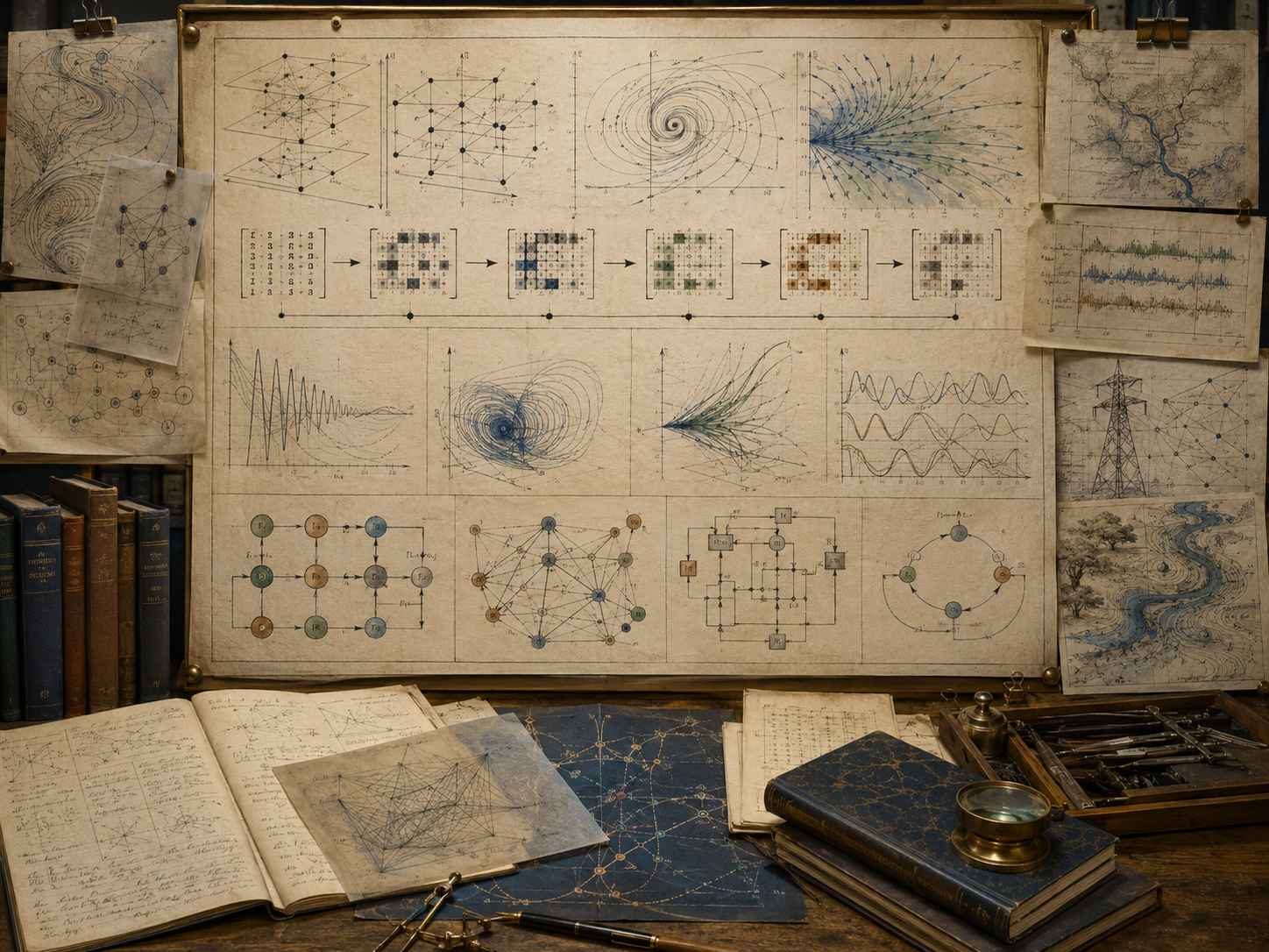
A matrix differential equation represents a continuous-time system using a state vector and a matrix of rate relationships. Each coordinate of the state may influence the rate of change of other coordinates. This makes the model useful for coupled physical systems, population dynamics, economic adjustment, infrastructure stress, signal processing, epidemiological approximations, control theory, and scientific computation.
The basic linear form is compact, but its implications can be deep. Eigenvalues classify whether modes decay, amplify, oscillate, or persist. Eigenvectors identify modal directions. The matrix exponential advances the state through time. Forced systems introduce external inputs. Numerical methods approximate trajectories when closed-form analysis is difficult. The modeler must keep the time interpretation, matrix construction, stability rule, and domain assumptions explicit.
Why Matrix Differential Equations Matter
Matrix differential equations matter because many systems change continuously rather than in isolated steps. Temperature, velocity, pressure, stress, concentration, capital adjustment, disease progression, population flow, control response, and signal dynamics often depend on rates of change. When several quantities change together, a matrix can organize how each variable affects the others.
Linear algebra makes continuous-time systems analyzable. A state vector records the current system condition. A derivative vector records the instantaneous rate of change. A matrix connects the current state to those rates. The resulting model can be solved, simulated, decomposed, stabilized, or criticized using matrix methods.
| Question | Matrix differential object | Systems interpretation |
|---|---|---|
| What is changing? | State vector \(\mathbf{x}(t)\) | System variables at time \(t\). |
| How fast is it changing? | Derivative vector \(\frac{d\mathbf{x}}{dt}\) | Instantaneous rates of change. |
| What couples the variables? | System matrix \(A\) | Linear rate relationships among state variables. |
| How does the state evolve? | Matrix exponential \(e^{At}\) | Continuous-time transition operator. |
| Does the system stabilize? | Eigenvalue real parts. | Modes decay, persist, oscillate, or amplify. |
Matrix differential equations turn continuous change into a structured linear algebra problem.
State Vectors and Rates of Change
A continuous-time state vector records the system at time \(t\):
\mathbf{x}(t)=
\begin{bmatrix}
x_1(t)\\
x_2(t)\\
\vdots\\
x_n(t)
\end{bmatrix}
\]
Interpretation: The state vector collects the system variables as functions of continuous time.
The derivative vector records instantaneous rates of change:
\frac{d\mathbf{x}}{dt}=
\begin{bmatrix}
\frac{dx_1}{dt}\\
\frac{dx_2}{dt}\\
\vdots\\
\frac{dx_n}{dt}
\end{bmatrix}
\]
Interpretation: The derivative vector describes how each state variable is changing at the current instant.
In systems modeling, state variables must be carefully chosen. Continuous-time models require units that make rate relationships meaningful. If a state variable is measured in dollars, people, tons, degrees, vehicles, infections, or stress units, its derivative has corresponding units per unit time.
| State design issue | Continuous-time concern | Modeling warning |
|---|---|---|
| Variable definition | What does each coordinate measure? | Ambiguous state variables produce ambiguous rate equations. |
| Units | What are the units per time? | Matrix entries inherit time-dependent units. |
| Time scale | Seconds, days, years, or another interval? | Continuous-time parameters depend on the time unit. |
| State completeness | Does the state contain enough information? | Hidden variables can make the apparent dynamics misleading. |
| Measurement noise | How reliable are state and derivative estimates? | Derivative estimation can amplify noise. |
A matrix differential equation begins with a state vector, but the state vector must be meaningful before the mathematics can be trusted.
The Basic Matrix Differential Equation
The basic homogeneous linear matrix differential equation is:
\frac{d\mathbf{x}}{dt}=A\mathbf{x}(t)
\]
Interpretation: The current state is transformed by matrix \(A\) to produce the instantaneous rate of change.
The matrix \(A\) is the system matrix. Its entries describe how each state variable contributes to each rate of change. In a two-variable system, this means:
\begin{bmatrix}
x_1′(t)\\
x_2′(t)
\end{bmatrix}
=
\begin{bmatrix}
a_{11} & a_{12}\\
a_{21} & a_{22}
\end{bmatrix}
\begin{bmatrix}
x_1(t)\\
x_2(t)
\end{bmatrix}
\]
Interpretation: Each derivative is a linear combination of the current state variables.
| Term | Formal role | Systems modeling meaning |
|---|---|---|
| \(\mathbf{x}(t)\) | State vector. | Current system condition. |
| \(\frac{d\mathbf{x}}{dt}\) | Rate vector. | Instantaneous direction and speed of change. |
| \(A\) | System matrix. | Coupling among state variables and rates. |
| \(a_{ij}\) | Matrix entry. | Contribution of state variable \(j\) to rate \(i\). |
| Homogeneous form | No external input. | System evolves only through internal state dependence. |
This compact equation is the continuous-time counterpart of discrete linear dynamics. It is simple enough to analyze and rich enough to capture many patterns of coupled system change.
Coupled Systems of Differential Equations
A matrix differential equation is a system of coupled scalar differential equations. For example:
\begin{aligned}
x_1′(t) &= a_{11}x_1(t)+a_{12}x_2(t)\\
x_2′(t) &= a_{21}x_1(t)+a_{22}x_2(t)
\end{aligned}
\]
Interpretation: The rate of each variable can depend on both variables, creating coupled dynamics.
Coupling is what makes matrix representation powerful. Instead of studying each equation separately, the modeler can study the system as one linear transformation from state to rate.
| Coupling pattern | Matrix structure | Systems interpretation |
|---|---|---|
| Independent variables | Diagonal matrix. | Each state changes without direct influence from others. |
| One-way influence | Triangular or asymmetric matrix. | One variable drives another without reciprocal feedback. |
| Mutual coupling | Off-diagonal entries in both directions. | Variables influence each other dynamically. |
| Positive feedback | Reinforcing signs and eigenvalues. | Amplification or instability may occur. |
| Balancing feedback | Opposing signs or damping structure. | Oscillation, stabilization, or regulation may occur. |
Matrix notation does not hide the equations; it organizes them so system-level behavior can be analyzed.
The Matrix Exponential
The solution to the homogeneous linear system is written using the matrix exponential:
\mathbf{x}(t)=e^{At}\mathbf{x}(0)
\]
Interpretation: The matrix exponential advances the initial state continuously through time.
The matrix exponential is defined by a power series:
e^{At}=I+At+\frac{(At)^2}{2!}+\frac{(At)^3}{3!}+\cdots
\]
Interpretation: The exponential of a matrix generalizes the scalar exponential to linear transformations.
This formula connects continuous-time dynamics to matrix powers. In discrete time, \(A^t\) advances the state by repeated steps. In continuous time, \(e^{At}\) advances the state by continuous flow.
| Object | Role | Interpretation |
|---|---|---|
| \(e^{At}\) | State transition operator. | Maps initial state to state at time \(t\). |
| \(I\) | Identity term. | No change at time zero. |
| \(At\) | First-order rate contribution. | Immediate linear change. |
| Higher powers | Repeated interaction terms. | Accumulated effects of coupled dynamics. |
| Numerical exponential | Computed approximation. | Requires stable algorithms for serious models. |
The matrix exponential is the continuous-time engine of linear dynamical analysis.
Eigenvalues and Continuous-Time Modes
Eigenvalues describe the modes of a matrix differential equation. If \(A\mathbf{v}=\lambda\mathbf{v}\), then along the eigenvector direction \(\mathbf{v}\), the solution behaves like:
\mathbf{x}(t)=e^{\lambda t}\mathbf{v}
\]
Interpretation: Along an eigenvector mode, continuous-time behavior is governed by the exponential \(e^{\lambda t}\).
This is the continuous-time counterpart of discrete-time modal behavior \(A^t\mathbf{v}=\lambda^t\mathbf{v}\). The difference is crucial: in continuous time, stability depends on the real part of eigenvalues, not on eigenvalue magnitude relative to one.
| Eigenvalue feature | Continuous-time behavior | Systems interpretation |
|---|---|---|
| \(\operatorname{Re}(\lambda)<0\) | Mode decays. | Disturbance fades along that mode. |
| \(\operatorname{Re}(\lambda)>0\) | Mode grows. | Instability or amplification occurs. |
| \(\operatorname{Re}(\lambda)=0\) | Boundary behavior. | Persistence, oscillation, or marginal behavior may occur. |
| Imaginary component | Oscillation. | Cyclic or rotating behavior appears. |
| Repeated eigenvalues | May involve generalized modes. | Jordan structure can add polynomial factors. |
Eigenvalues convert a coupled continuous-time system into modal growth, decay, and oscillation patterns.
Continuous-Time Stability
For the homogeneous system \(\frac{d\mathbf{x}}{dt}=A\mathbf{x}\), asymptotic stability generally requires all eigenvalues of \(A\) to have negative real parts:
\operatorname{Re}(\lambda_i)<0
\quad \text{for all eigenvalues } \lambda_i
\]
Interpretation: If all modes decay exponentially, the continuous-time system is asymptotically stable around the zero equilibrium.
This differs from discrete-time stability, where eigenvalues must lie inside the unit circle. The same numeric matrix can mean different things depending on whether it is interpreted as a discrete update matrix or as a continuous-time generator.
| Eigenvalue condition | Continuous-time implication | Systems interpretation |
|---|---|---|
| All real parts negative | Asymptotic decay. | Disturbances fade toward equilibrium. |
| Any real part positive | Instability. | Some disturbance mode amplifies. |
| Real part equal to zero | Boundary behavior. | Persistence or oscillation may require deeper analysis. |
| Complex pair with negative real part | Damped oscillation. | Cyclic behavior fades over time. |
| Complex pair with positive real part | Growing oscillation. | Cycles amplify and may become unstable. |
Continuous-time stability should always be reported with the time interpretation of the matrix. A matrix used as a generator is not the same kind of object as a one-step transition matrix.
Diagonalization and Decoupling
If the system matrix is diagonalizable, it can be written as:
A=PDP^{-1}
\]
Interpretation: The matrix \(A\) can be represented in an eigenvector basis where \(D\) contains eigenvalues on the diagonal.
The matrix exponential becomes:
e^{At}=Pe^{Dt}P^{-1}
\]
Interpretation: In modal coordinates, the system evolves through independent scalar exponentials.
Because \(D\) is diagonal:
e^{Dt}=
\begin{bmatrix}
e^{\lambda_1t} & 0 & \cdots & 0\\
0 & e^{\lambda_2t} & \cdots & 0\\
\vdots & \vdots & \ddots & \vdots\\
0 & 0 & \cdots & e^{\lambda_nt}
\end{bmatrix}
\]
Interpretation: Each decoupled mode evolves according to its own exponential rate.
| Diagonalization object | Role | Systems interpretation |
|---|---|---|
| \(P\) | Eigenvector matrix. | Transforms original variables into modal coordinates. |
| \(D\) | Diagonal eigenvalue matrix. | Separates independent modal rates. |
| \(e^{Dt}\) | Diagonal exponential. | Each mode grows, decays, or oscillates independently. |
| \(Pe^{Dt}P^{-1}\) | Return to original coordinates. | Combines modal behavior into observable system variables. |
| Conditioning of \(P\) | Sensitivity of modal basis. | Ill-conditioned eigenvectors make modal interpretation fragile. |
Diagonalization can make matrix differential equations interpretable, but only when the modal basis is valid, well-conditioned, and meaningful for the system.
Oscillation and Complex Eigenvalues
Complex eigenvalues naturally produce oscillatory behavior. If an eigenvalue has the form:
\lambda=\alpha+i\beta
\]
Interpretation: The real part \(\alpha\) controls growth or decay, while the imaginary part \(\beta\) controls oscillation.
The corresponding exponential is:
e^{(\alpha+i\beta)t}=e^{\alpha t}(\cos(\beta t)+i\sin(\beta t))
\]
Interpretation: Complex eigenvalues combine exponential scaling with rotational oscillation.
| Complex eigenvalue type | Dynamic behavior | Systems interpretation |
|---|---|---|
| \(\alpha<0\) | Damped oscillation. | Cycles fade toward equilibrium. |
| \(\alpha=0\) | Persistent oscillation. | Idealized undamped cycling may occur. |
| \(\alpha>0\) | Growing oscillation. | Instability with cyclic amplification. |
| Large \(|\beta|\) | Faster oscillation. | Shorter cycle period. |
| Small \(|\alpha|\) | Slow damping or slow growth. | Long transient behavior may matter. |
Oscillatory modes are common in systems with exchange, feedback, inertia, predator-prey approximation, economic adjustment, control loops, and physical motion.
Forced Matrix Differential Equations
Many systems include external input, forcing, intervention, or control. A forced linear matrix differential equation has the form:
\frac{d\mathbf{x}}{dt}=A\mathbf{x}(t)+\mathbf{b}(t)
\]
Interpretation: The system changes through internal linear dynamics plus an external time-dependent input.
With an input matrix, the state-space form is:
\frac{d\mathbf{x}}{dt}=A\mathbf{x}(t)+B\mathbf{u}(t)
\]
Interpretation: The input vector \(\mathbf{u}(t)\) affects the state through input matrix \(B\).
The solution includes both the natural response and the accumulated forced response:
\mathbf{x}(t)=e^{At}\mathbf{x}(0)+\int_0^t e^{A(t-\tau)}\mathbf{b}(\tau)\,d\tau
\]
Interpretation: The state combines the unforced evolution of the initial condition with the accumulated effect of external forcing.
| Term | Role | Systems interpretation |
|---|---|---|
| \(e^{At}\mathbf{x}(0)\) | Natural response. | Evolution caused by the initial condition. |
| \(\mathbf{b}(t)\) | External forcing. | Shock, intervention, background input, or environmental driver. |
| \(B\mathbf{u}(t)\) | Controlled input. | Decision or control signal entering through specified channels. |
| Integral term | Accumulated input response. | How past inputs continue to affect current state. |
| Input validation | Model audit requirement. | Forcing assumptions require their own evidence and uncertainty review. |
Forced matrix differential equations lead naturally into control systems modeling, where input design, response, controllability, observability, and stabilization become central.
Equilibrium and Steady State
An equilibrium occurs when the derivative is zero. For the homogeneous system:
A\mathbf{x}^\ast=\mathbf{0}
\]
Interpretation: At equilibrium, the state produces no instantaneous change.
For a constant forced system:
\frac{d\mathbf{x}}{dt}=A\mathbf{x}+\mathbf{b}
\]
Interpretation: The system has internal dynamics plus constant external input.
An equilibrium satisfies:
A\mathbf{x}^\ast+\mathbf{b}=\mathbf{0}
\]
Interpretation: At equilibrium, internal dynamics and external input balance.
If \(A\) is invertible, then:
\mathbf{x}^\ast=-A^{-1}\mathbf{b}
\]
Interpretation: The steady state can be recovered by solving a linear system.
| Equilibrium question | Mathematical test | Systems interpretation |
|---|---|---|
| Does equilibrium exist? | Solve \(A\mathbf{x}^\ast+\mathbf{b}=0\). | Can the system balance internal dynamics and forcing? |
| Is it unique? | Check invertibility or rank. | Multiple equilibria or no equilibrium may be possible. |
| Is it stable? | Check eigenvalue real parts. | Do nearby states return or move away? |
| Is it feasible? | Check constraints and units. | The algebraic equilibrium must make domain sense. |
| Is it desirable? | Domain and governance review. | Stable does not mean equitable, safe, resilient, or acceptable. |
Equilibrium is a mathematical condition. Its meaning depends on the system, units, constraints, and values attached to the modeled state.
Fundamental Matrix Solutions
A fundamental matrix solution organizes a full set of independent solutions into a matrix. For the homogeneous system:
\frac{d\mathbf{x}}{dt}=A\mathbf{x}
\]
Interpretation: The homogeneous system describes all natural system responses without forcing.
A fundamental matrix \(\Phi(t)\) satisfies:
\Phi'(t)=A\Phi(t)
\]
Interpretation: Each column of \(\Phi(t)\) is a solution trajectory of the system.
When \(\Phi(0)=I\), the fundamental matrix is the matrix exponential:
\Phi(t)=e^{At}
\]
Interpretation: The matrix exponential is the fundamental transition matrix starting from identity.
| Object | Meaning | Use |
|---|---|---|
| Fundamental matrix | Matrix of independent solutions. | Describes all homogeneous trajectories. |
| Initial identity condition | \(\Phi(0)=I\) | Turns the fundamental matrix into a state transition matrix. |
| State transition matrix | Maps \(\mathbf{x}(0)\) to \(\mathbf{x}(t)\). | Advances initial states through continuous time. |
| Invertibility | Independent solution columns. | Ensures the solution basis spans the state space. |
| Time-varying extension | \(A(t)\) instead of constant \(A\). | More complex systems require time-ordered or numerical treatment. |
Fundamental matrices generalize the idea of using a basis to describe all possible system trajectories.
Discrete Versus Continuous Time
Discrete-time and continuous-time linear systems are related but not interchangeable. Discrete systems update by steps:
\mathbf{x}_{t+1}=A\mathbf{x}_t
\]
Interpretation: The state changes at distinct time steps through multiplication by \(A\).
Continuous systems evolve through rates:
\frac{d\mathbf{x}}{dt}=A\mathbf{x}(t)
\]
Interpretation: The state changes continuously according to a rate determined by \(A\).
Their evolution operators differ:
\text{discrete: } A^t,
\qquad
\text{continuous: } e^{At}
\]
Interpretation: Discrete systems use matrix powers; continuous systems use matrix exponentials.
| Feature | Discrete-time system | Continuous-time system |
|---|---|---|
| Equation | \(\mathbf{x}_{t+1}=A\mathbf{x}_t\) | \(\frac{d\mathbf{x}}{dt}=A\mathbf{x}\) |
| Evolution operator | \(A^t\) | \(e^{At}\) |
| Stability rule | Eigenvalues inside unit circle. | Eigenvalue real parts negative. |
| Time interpretation | Step index or interval. | Continuous time variable. |
| Parameter meaning | Per-step multiplier. | Per-time-unit rate. |
Confusing discrete and continuous interpretations is one of the most serious errors in matrix dynamics. The matrix’s meaning changes with the time model.
Numerical Simulation and Stiffness
Matrix differential equations can sometimes be solved analytically, but computation is often necessary. Numerical workflows may compute the matrix exponential directly, integrate the system using ordinary differential equation solvers, or simulate forced systems over time.
Numerical reliability matters. Some systems are stiff: they contain fast and slow modes together. A stiff system may be stable in theory but difficult to simulate accurately with naive time-stepping methods.
| Numerical issue | Why it matters | Modeling response |
|---|---|---|
| Matrix exponential accuracy | Direct computation can be sensitive for some matrices. | Use reliable library routines and residual checks. |
| Step size | Large steps can distort continuous dynamics. | Use adaptive solvers or justified discretization. |
| Stiffness | Fast and slow modes create simulation difficulty. | Use stiff solvers and inspect eigenvalue scales. |
| Nonnormality | Short-run growth can occur despite stable eigenvalues. | Track trajectory norms and transient amplification. |
| Conditioning | Eigenvectors and exponentials can be sensitive. | Review perturbation sensitivity and numerical diagnostics. |
| Constraint violation | Linear ODEs may produce impossible states. | Check nonnegativity, capacity, conservation, and domain bounds. |
Numerical simulation should be treated as part of the model audit, not merely as a way to produce plots.
Matrix Differential Equations in Systems Modeling
Matrix differential equations are useful when system variables change continuously and interact through approximately linear rates. They can describe physical motion, engineering response, control systems, economic adjustment, ecological coupling, epidemiological approximations, chemical systems, infrastructure stress, financial dynamics, signal processing, and scientific computation.
The same form can represent different modeling commitments. In one context, \(A\) may be derived from physical law. In another, it may be estimated from data. In another, it may be a local Jacobian near equilibrium. In another, it may be an exploratory scenario matrix. These are not equivalent uses.
| Domain | Matrix differential use | Interpretive caution |
|---|---|---|
| Engineering | Continuous state-space response and control. | Inputs, outputs, constraints, and uncertainty matter. |
| Ecology | Linearized population or interaction dynamics. | Carrying capacity, thresholds, and nonlinear feedback may dominate. |
| Economics | Continuous adjustment among coupled variables. | Behavioral and institutional changes can alter rates. |
| Infrastructure | Stress, degradation, and service dynamics. | Failure thresholds may be nonlinear and discontinuous. |
| Public health | Compartment approximations and local dynamics. | Contact behavior and intervention effects can be time-varying. |
| Scientific computing | Linear ODE systems, discretized PDEs, and solver tests. | Stiffness, conditioning, and step-size control are essential. |
Matrix differential equations are powerful because they make coupled continuous change mathematically transparent. They are risky when the transparency is mistaken for completeness.
Mathematical Deepening
This section adds a more formal layer. Matrix differential equations connect linear ordinary differential equations, state-space representation, matrix exponentials, eigenvalues, eigenvectors, diagonalization, Jordan forms, fundamental matrices, variation of constants, stability theory, stiff systems, numerical integration, local linearization, controllability, observability, and model validation.
Continuous-Time Structure Review
State Vector
The state vector records system variables as functions of continuous time.
Derivative Vector
The derivative vector records instantaneous rates of change.
System Matrix
The system matrix maps current state into current rate of change.
Time Units
Continuous-time matrix entries are rate parameters and depend on the chosen time unit.
Matrix Exponential Review
State Transition
The matrix exponential advances the state through continuous time.
Modal Exponentials
Eigenvalues generate scalar exponentials that govern modal behavior.
Diagonalization
When valid, diagonalization separates the system into independent continuous-time modes.
Numerical Exponential
Reliable computation requires stable algorithms, not naive power-series truncation.
Stability Review
Negative Real Parts
Continuous-time asymptotic stability requires eigenvalue real parts to be negative.
Boundary Modes
Eigenvalues on the imaginary axis require deeper analysis of persistence or oscillation.
Complex Modes
Complex eigenvalues produce oscillatory behavior with damping or growth set by real parts.
Nonnormality
Stable eigenvalues may still allow short-run transient amplification in nonnormal systems.
Forced Response Review
Natural Response
The initial condition evolves through the matrix exponential.
Input Response
External forcing contributes through accumulated transformed inputs.
Equilibrium Balance
Constant forcing can create a nonzero equilibrium when the linear system is solvable.
Control Preview
Input matrices prepare the transition to control systems modeling.
Governance Questions
What Does the Matrix Measure?
Matrix entries should have rate meaning, units, and documented source.
Why Continuous Time?
The model should justify why continuous evolution is more appropriate than discrete updates.
Is the System Truly Linear?
The model should clarify whether linearity is structural, local, empirical, or exploratory.
What Is the Valid Horizon?
A matrix differential equation may be valid only near an equilibrium or over a specific time range.
Examples from Systems Modeling
Matrix differential equations appear whenever coupled state variables evolve continuously through linear or locally linear rate relationships.
Engineering State-Space Systems
Position, velocity, current, voltage, pressure, or temperature states can evolve continuously through matrices derived from physical laws.
Infrastructure Stress Dynamics
Coupled service, load, delay, and degradation variables can be approximated by continuous-time stress propagation models.
Ecological Linearization
Nonlinear ecological systems can be locally approximated near equilibrium using a Jacobian matrix and continuous-time stability analysis.
Economic Adjustment
Capital, demand, price, production, or sector variables can be modeled as continuously adjusting through coupled rate equations.
Public Health Compartments
Linearized compartment models can approximate local disease dynamics, recovery, exposure, or intervention response.
Scientific Computing and PDE Discretization
Spatially discretized partial differential equations often produce large systems of matrix differential equations requiring careful numerical integration.
Across these examples, continuous-time matrix dynamics should be interpreted through units, time scale, stability, forcing, numerical reliability, and domain validity.
Computation and Reproducible Workflows
Computational workflows for matrix differential equations should document the state variables, units, time scale, system matrix, initial condition, eigenvalues, real parts, stability classification, matrix exponential or numerical solver, trajectory horizon, forced inputs, equilibrium checks, stiffness diagnostics, constraint checks, sensitivity tests, and interpretation warnings.
The companion repository treats matrix differential equations as auditable continuous-time systems models. Python, R, Julia, SQL, Haskell, C, C++, Fortran, Rust, Go, notebooks, schemas, generated outputs, Canvas artifacts, advanced reports, and calculators each support a different layer of reproducible continuous-time linear dynamics analysis.
For this article, the computational examples focus on matrix-exponential intuition, eigenvalue real-part stability, trajectory diagnostics, equilibrium review, stiffness warnings, and governance records for continuous-time model claims.
Python Workflow: Matrix Differential Equation Audit
The Python workflow below audits a two-state continuous-time system, computes real eigenvalues for a teaching matrix, classifies continuous-time stability by eigenvalue real parts, simulates a simple closed-form trajectory for diagonalizable real modes, and writes reproducible outputs.
from __future__ import annotations

from dataclasses import asdict, dataclass
from pathlib import Path
import csv
import json
import math


Matrix = list[list[float]]
Vector = list[float]


@dataclass(frozen=True)
class MatrixDifferentialAudit:
    system_name: str
    state_names: str
    system_matrix: str
    initial_state: str
    time_horizon: float
    eigenvalue_1: float
    eigenvalue_2: float
    max_real_part: float
    stability_classification: str
    final_state_estimate: str
    initial_norm: float
    final_norm: float
    time_model_warning: str
    interpretation_warning: str


def matrix_to_string(A: Matrix) -> str:
    return ";".join(",".join(f"{value:.6f}" for value in row) for row in A)


def vector_to_string(x: Vector) -> str:
    return ",".join(f"{value:.6f}" for value in x)


def norm2(x: Vector) -> float:
    return math.sqrt(sum(value * value for value in x))


def trace_2x2(A: Matrix) -> float:
    return A[0][0] + A[1][1]


def determinant_2x2(A: Matrix) -> float:
    return A[0][0] * A[1][1] - A[0][1] * A[1][0]


def eigenvalues_2x2_real(A: Matrix) -> tuple[float, float]:
    trace = trace_2x2(A)
    determinant = determinant_2x2(A)
    discriminant = trace * trace - 4.0 * determinant
    if discriminant < 0:
        raise ValueError("This teaching routine handles real eigenvalues only.")
    root = math.sqrt(discriminant)
    return ((trace + root) / 2.0, (trace - root) / 2.0)


def classify_continuous(max_real_part: float) -> str:
    if max_real_part < 0.0:
        return "asymptotically_stable_continuous_time"
    if abs(max_real_part) <= 1e-10:
        return "boundary_or_marginal_continuous_time"
    return "unstable_continuous_time"


def matvec(A: Matrix, x: Vector) -> Vector:
    return [sum(A[i][j] * x[j] for j in range(len(x))) for i in range(len(A))]


def euler_simulate(A: Matrix, x0: Vector, horizon: float, dt: float) -> Vector:
    steps = int(round(horizon / dt))
    x = x0[:]
    for _ in range(steps):
        dx = matvec(A, x)
        x = [x[i] + dt * dx[i] for i in range(len(x))]
    return x


def build_audit() -> MatrixDifferentialAudit:
    state_names = ["infrastructure_stress", "service_delay"]

    # Continuous-time generator-style matrix:
    # negative diagonal damping with positive cross-coupling.
    A = [
        [-0.28, 0.08],
        [0.12, -0.34],
    ]

    x0 = [10.0, 4.0]
    horizon = 10.0
    dt = 0.01

    eigenvalues = eigenvalues_2x2_real(A)
    max_real_part = max(eigenvalues)
    final_state = euler_simulate(A, x0, horizon, dt)

    return MatrixDifferentialAudit(
        system_name="two_state_matrix_differential_equation_audit",
        state_names="|".join(state_names),
        system_matrix=matrix_to_string(A),
        initial_state=vector_to_string(x0),
        time_horizon=horizon,
        eigenvalue_1=round(eigenvalues[0], 12),
        eigenvalue_2=round(eigenvalues[1], 12),
        max_real_part=round(max_real_part, 12),
        stability_classification=classify_continuous(max_real_part),
        final_state_estimate=vector_to_string(final_state),
        initial_norm=round(norm2(x0), 12),
        final_norm=round(norm2(final_state), 12),
        time_model_warning=(
            "This matrix is interpreted as a continuous-time generator. "
            "Do not apply discrete-time spectral-radius rules to it."
        ),
        interpretation_warning=(
            "Matrix differential equations depend on state definitions, units, time scale, "
            "matrix source, linearity assumptions, solver choices, stiffness review, and domain constraints."
        ),
    )


def write_outputs(output_dir: Path) -> None:
    (output_dir / "tables").mkdir(parents=True, exist_ok=True)
    (output_dir / "json").mkdir(parents=True, exist_ok=True)

    audit = build_audit()
    row = asdict(audit)

    with (output_dir / "tables" / "matrix_differential_equation_audit.csv").open(
        "w", newline="", encoding="utf-8"
    ) as handle:
        writer = csv.DictWriter(handle, fieldnames=list(row.keys()))
        writer.writeheader()
        writer.writerow(row)

    (output_dir / "json" / "matrix_differential_equation_audit.json").write_text(
        json.dumps(row, indent=2, sort_keys=True),
        encoding="utf-8",
    )


if __name__ == "__main__":
    write_outputs(Path("outputs"))
    print("Matrix differential equation audit complete.")
This workflow keeps the continuous-time interpretation, eigenvalue real-part classification, trajectory estimate, and modeling warnings together.
R Workflow: Continuous-Time Stability Diagnostics
R can support matrix differential equation diagnostics by computing eigenvalues, classifying continuous-time stability, and simulating a trajectory with a simple numerical method.
A <- matrix(
  c(
    -0.28, 0.08,
     0.12, -0.34
  ),
  nrow = 2,
  byrow = TRUE
)

state_names <- c("infrastructure_stress", "service_delay")
x0 <- c(10.0, 4.0)
horizon <- 10.0
dt <- 0.01
steps <- as.integer(round(horizon / dt))

trajectory <- matrix(NA, nrow = steps + 1, ncol = length(x0))
trajectory[1, ] <- x0

for (k in seq_len(steps)) {
  dx <- A %*% trajectory[k, ]
  trajectory[k + 1, ] <- trajectory[k, ] + dt * as.numeric(dx)
}

state_norms <- apply(trajectory, 1, function(row) sqrt(sum(row^2)))
eigen_values <- eigen(A)$values
max_real_part <- max(Re(eigen_values))

stability_classification <- ifelse(
  max_real_part < 0,
  "asymptotically_stable_continuous_time",
  ifelse(abs(max_real_part) <= 1e-10, "boundary_or_marginal_continuous_time", "unstable_continuous_time")
)

audit_record <- data.frame(
  system_name = "two_state_matrix_differential_equation_audit",
  state_names = paste(state_names, collapse = "|"),
  system_matrix = paste(round(as.vector(t(A)), 6), collapse = ","),
  initial_state = paste(round(x0, 6), collapse = ","),
  time_horizon = horizon,
  final_state_estimate = paste(round(trajectory[steps + 1, ], 6), collapse = ","),
  initial_norm = state_norms[1],
  final_norm = state_norms[steps + 1],
  eigenvalues = paste(round(Re(eigen_values), 6), collapse = ","),
  max_real_part = max_real_part,
  stability_classification = stability_classification,
  interpretation_warning = paste(
    "Matrix differential equations require continuous-time stability rules,",
    "time-scale clarity, solver review, stiffness checks, and domain interpretation."
  )
)

dir.create("outputs/tables", recursive = TRUE, showWarnings = FALSE)

write.csv(
  audit_record,
  "outputs/tables/r_matrix_differential_equation_audit.csv",
  row.names = FALSE
)

trajectory_record <- data.frame(
  time = seq(0, horizon, by = dt),
  infrastructure_stress = trajectory[, 1],
  service_delay = trajectory[, 2],
  state_norm = state_norms
)

write.csv(
  trajectory_record,
  "outputs/tables/r_matrix_differential_equation_trajectory.csv",
  row.names = FALSE
)

print(audit_record)
This R workflow makes continuous-time stability and finite-horizon trajectory behavior auditable as data.
Haskell Workflow: Typed Continuous-Time Records
Haskell can represent matrix differential equation diagnostics as typed records, keeping continuous-time interpretation, stability classification, and domain warnings explicit.
module Main where

data MatrixDifferentialAudit = MatrixDifferentialAudit
  { systemName :: String
  , stateNames :: String
  , systemMatrix :: String
  , initialState :: String
  , timeHorizon :: Double
  , eigenvalues :: String
  , maxRealPart :: Double
  , stabilityClassification :: String
  , finalStateEstimate :: String
  , interpretationWarning :: String
  } deriving (Show)

buildAudit :: MatrixDifferentialAudit
buildAudit =
  MatrixDifferentialAudit
    "two_state_matrix_differential_equation_audit"
    "infrastructure_stress|service_delay"
    "-0.280000,0.080000;0.120000,-0.340000"
    "10.000000,4.000000"
    10.0
    "-0.200000,-0.420000"
    (-0.20)
    "asymptotically_stable_continuous_time"
    "1.558000,0.882000"
    "Matrix differential equations depend on state definitions, units, time scale, solver choices, stiffness review, and domain constraints."

main :: IO ()
main =
  print buildAudit
The typed workflow helps prevent a common modeling error: treating a continuous-time generator as though it were a discrete-time transition matrix.
SQL Workflow: Matrix Differential Equation Assumption Registry
SQL can document continuous-time modeling assumptions when matrix differential equations support dashboards, simulations, engineering review, infrastructure planning, public-health modeling, scientific workflows, or institutional decision systems.
CREATE TABLE matrix_differential_assumption_registry (
    assumption_key TEXT PRIMARY KEY,
    assumption_name TEXT NOT NULL,
    mathematical_role TEXT NOT NULL,
    systems_modeling_role TEXT NOT NULL,
    review_warning TEXT NOT NULL
);

INSERT INTO matrix_differential_assumption_registry VALUES
(
  'state_vector',
  'State vector',
  'Defines the coordinates of continuous-time system state.',
  'Determines what the model can track through time.',
  'State variables require units, scales, and domain definitions.'
);

INSERT INTO matrix_differential_assumption_registry VALUES
(
  'system_matrix',
  'System matrix',
  'Maps current state into instantaneous rate of change.',
  'Encodes rate coupling among variables.',
  'Matrix entries are rate parameters and require time-unit clarity.'
);

INSERT INTO matrix_differential_assumption_registry VALUES
(
  'continuous_time',
  'Continuous-time interpretation',
  'Uses dx/dt = Ax rather than x_{t+1} = Ax_t.',
  'Determines the correct evolution operator and stability rule.',
  'Do not apply discrete-time spectral-radius rules to a continuous-time generator.'
);

INSERT INTO matrix_differential_assumption_registry VALUES
(
  'matrix_exponential',
  'Matrix exponential',
  'Advances the initial state through continuous time.',
  'Represents the continuous state transition operator.',
  'Numerical computation of exp(At) should use reliable algorithms.'
);

INSERT INTO matrix_differential_assumption_registry VALUES
(
  'stability',
  'Continuous-time stability',
  'Classifies modes using eigenvalue real parts.',
  'Shows whether disturbances decay, persist, oscillate, or amplify.',
  'Stable eigenvalues do not automatically imply practical safety or desirability.'
);

INSERT INTO matrix_differential_assumption_registry VALUES
(
  'solver_review',
  'Solver review',
  'Checks numerical integration method, step size, and stiffness.',
  'Determines whether simulated trajectories are reliable.',
  'Naive time stepping can distort stiff or sensitive continuous systems.'
);

SELECT
    assumption_name,
    mathematical_role,
    systems_modeling_role,
    review_warning
FROM matrix_differential_assumption_registry
ORDER BY assumption_key;
This registry keeps matrix differential equation analysis tied to state design, rate interpretation, continuous-time stability, matrix exponentials, solver reliability, and responsible interpretation.
GitHub Repository
The companion repository for this article is designed as a reproducible mathematical-modeling workspace. It supports matrix differential equation audits, continuous-time stability diagnostics, eigenvalue real-part reports, matrix-exponential interpretation, trajectory simulation, solver review, SQL governance tables, generated outputs, advanced mathematical audit reports, and reusable calculator scripts.
Complete Code Repository
Companion article folder with Python, R, Julia, SQL, Haskell, C, C++, Fortran, Rust, Go, notebooks, documentation, synthetic teaching data, generated outputs, schemas, Canvas-ready workflow artifacts, and reusable calculator scripts for matrix differential equations, continuous-time linear dynamics, state vectors, derivative vectors, system matrices, matrix exponentials, eigenvalue stability, forced response, equilibrium analysis, numerical simulation, solver diagnostics, model governance, and responsible mathematical modeling.
Interpretive Limits and Responsible Use
Matrix differential equations are powerful because they make continuous coupled change mathematically tractable. They can reveal modal structure, damping, amplification, oscillation, equilibrium, forced response, and stability. Their limits arise because real systems may be nonlinear, threshold-driven, constrained, adaptive, discontinuous, stochastic, delayed, spatially heterogeneous, or institutionally shaped.
A matrix differential equation may represent a physical law, an engineering state-space model, a local Jacobian approximation, an empirical continuous-time fit, a simplified policy model, or a scenario abstraction. These uses require different evidence. A model derived from conservation laws is different from a matrix estimated from sparse observational data. A local linearization near equilibrium is different from a global claim about the whole system.
Responsible use requires documenting state variables, units, time scale, matrix source, rate interpretation, initial conditions, forcing terms, equilibrium assumptions, eigenvalues, stability classification, numerical solver, stiffness diagnostics, constraint checks, uncertainty, sensitivity tests, and the practical horizon over which the linear continuous-time model should be trusted. Matrix differential equations should clarify continuous dynamics without pretending that linear rates fully describe complex systems.
Related Articles
- What Is Linear Algebra for Systems Modeling?
- Scalars, Vectors, and System States
- Vector Spaces and System Representation
- Span, Linear Independence, and Basis
- Dimension and the Structure of Solution Spaces
- Matrices and the Organization of Multivariable Systems
- Matrix Arithmetic and the Logic of Combination
- Systems of Linear Equations
- Gaussian Elimination and Row Reduction
- Pivot Structure and Solvability
- Rank, Nullity, and Structural Dependence
- Determinants and Invertibility
- Inverse Matrices and Structural Recovery
- Overdetermined Systems and Least Squares Thinking
- Linear Transformations and Model Behavior
- Matrix Multiplication and Interaction Effects
- Change of Basis and Alternative Representations
- Projections, Reflections, and Geometric Interpretation
- Orthogonality and Structured Simplification
- Inner Products, Norms, and Distance in State Space
- Eigenvalues, Eigenvectors, and System Modes
- Diagonalization and Decoupled System Behavior
- Stability Analysis with Eigenvalues
- Markov Chains and Transition Matrices
- Long-Run Behavior in State Transition Systems
- Linear Dynamical Systems
- Linear Algebra for Systems Modeling
- Mathematical Modeling
- Systems Modeling
- Differential Equations for Systems Modeling
- Scientific Computing for Systems Modeling
Further Reading
- Boyd, S. and Vandenberghe, L. (2018) Introduction to Applied Linear Algebra: Vectors, Matrices, and Least Squares. Cambridge: Cambridge University Press. Available at: https://vmls-book.stanford.edu/.
- Chen, C.-T. (1999) Linear System Theory and Design. 3rd edn. Oxford: Oxford University Press. Available at: https://global.oup.com/academic/product/linear-system-theory-and-design-9780195117776.
- Georgia Institute of Technology (n.d.) Interactive Linear Algebra. Georgia Institute of Technology. Available at: https://textbooks.math.gatech.edu/ila/.
- Golub, G.H. and Van Loan, C.F. (2013) Matrix Computations. 4th edn. Baltimore, MD: Johns Hopkins University Press. Available at: https://www.press.jhu.edu/books/title/10678/matrix-computations.
- Hirsch, M.W., Smale, S. and Devaney, R.L. (2013) Differential Equations, Dynamical Systems, and an Introduction to Chaos. 3rd edn. Amsterdam: Academic Press. Available at: https://www.elsevier.com/books/differential-equations-dynamical-systems-and-an-introduction-to-chaos/hirsch/978-0-12-382010-5.
- Higham, N.J. (2008) Functions of Matrices: Theory and Computation. Philadelphia, PA: Society for Industrial and Applied Mathematics. Available at: https://epubs.siam.org/doi/book/10.1137/1.9780898717778.
- Higham, N.J. (2002) Accuracy and Stability of Numerical Algorithms. 2nd edn. Philadelphia, PA: Society for Industrial and Applied Mathematics. Available at: https://epubs.siam.org/doi/book/10.1137/1.9780898718027.
- Horn, R.A. and Johnson, C.R. (2013) Matrix Analysis. 2nd edn. Cambridge: Cambridge University Press. Available at: https://www.cambridge.org/highereducation/books/matrix-analysis/FDA3627DC2B9F5C3DF2FD8C3CC136B48.
- Kailath, T. (1980) Linear Systems. Englewood Cliffs, NJ: Prentice Hall. Available at: https://archive.org/details/linearsystems0000kail.
- Khalil, H.K. (2002) Nonlinear Systems. 3rd edn. Upper Saddle River, NJ: Prentice Hall. Available at: https://www.egr.msu.edu/~khalil/NonlinearSystems/.
- Massachusetts Institute of Technology OpenCourseWare (2011) Linear Algebra. Cambridge, MA: MIT OpenCourseWare. Available at: https://ocw.mit.edu/courses/18-06sc-linear-algebra-fall-2011/.
- Massachusetts Institute of Technology OpenCourseWare (2011) Dynamic Systems and Control. Cambridge, MA: MIT OpenCourseWare. Available at: https://ocw.mit.edu/courses/6-241j-dynamic-systems-and-control-spring-2011/.
- Massachusetts Institute of Technology OpenCourseWare (2014) Differential Equations. Cambridge, MA: MIT OpenCourseWare. Available at: https://ocw.mit.edu/courses/18-03sc-differential-equations-fall-2011/.
- Meyer, C.D. (2023) Matrix Analysis and Applied Linear Algebra. 2nd edn. Philadelphia, PA: Society for Industrial and Applied Mathematics. Available at: https://epubs.siam.org/doi/book/10.1137/1.9781611977448.
- Netlib (n.d.) LAPACK — Linear Algebra PACKage. Netlib Repository. Available at: https://www.netlib.org/lapack/.
- NumPy Developers (n.d.) Linear Algebra: numpy.linalg. NumPy Documentation. Available at: https://numpy.org/doc/stable/reference/routines.linalg.html.
- SciPy Developers (n.d.) Integration and ODEs: scipy.integrate. SciPy Documentation. Available at: https://docs.scipy.org/doc/scipy/reference/integrate.html.
- SciPy Developers (n.d.) Matrix Exponential: scipy.linalg.expm. SciPy Documentation. Available at: https://docs.scipy.org/doc/scipy/reference/generated/scipy.linalg.expm.html.
- Strogatz, S.H. (2018) Nonlinear Dynamics and Chaos. 2nd edn. Boca Raton, FL: CRC Press. Available at: https://www.routledge.com/Nonlinear-Dynamics-and-Chaos-With-Applications-to-Physics-Biology-Chemistry-and-Engineering/Strogatz/p/book/9780813349107.
- Trefethen, L.N. and Bau, D. (1997) Numerical Linear Algebra. Philadelphia, PA: Society for Industrial and Applied Mathematics. Available at: https://epubs.siam.org/doi/book/10.1137/1.9780898719574.
References
- Boyd, S. and Vandenberghe, L. (2018) Introduction to Applied Linear Algebra: Vectors, Matrices, and Least Squares. Cambridge: Cambridge University Press. Available at: https://vmls-book.stanford.edu/.
- Chen, C.-T. (1999) Linear System Theory and Design. 3rd edn. Oxford: Oxford University Press. Available at: https://global.oup.com/academic/product/linear-system-theory-and-design-9780195117776.
- Golub, G.H. and Van Loan, C.F. (2013) Matrix Computations. 4th edn. Baltimore, MD: Johns Hopkins University Press. Available at: https://www.press.jhu.edu/books/title/10678/matrix-computations.
- Hirsch, M.W., Smale, S. and Devaney, R.L. (2013) Differential Equations, Dynamical Systems, and an Introduction to Chaos. 3rd edn. Amsterdam: Academic Press. Available at: https://www.elsevier.com/books/differential-equations-dynamical-systems-and-an-introduction-to-chaos/hirsch/978-0-12-382010-5.
- Higham, N.J. (2008) Functions of Matrices: Theory and Computation. Philadelphia, PA: Society for Industrial and Applied Mathematics. Available at: https://epubs.siam.org/doi/book/10.1137/1.9780898717778.
- Higham, N.J. (2002) Accuracy and Stability of Numerical Algorithms. 2nd edn. Philadelphia, PA: Society for Industrial and Applied Mathematics. Available at: https://epubs.siam.org/doi/book/10.1137/1.9780898718027.
- Horn, R.A. and Johnson, C.R. (2013) Matrix Analysis. 2nd edn. Cambridge: Cambridge University Press. Available at: https://www.cambridge.org/highereducation/books/matrix-analysis/FDA3627DC2B9F5C3DF2FD8C3CC136B48.
- Kailath, T. (1980) Linear Systems. Englewood Cliffs, NJ: Prentice Hall. Available at: https://archive.org/details/linearsystems0000kail.
- Khalil, H.K. (2002) Nonlinear Systems. 3rd edn. Upper Saddle River, NJ: Prentice Hall. Available at: https://www.egr.msu.edu/~khalil/NonlinearSystems/.
- Massachusetts Institute of Technology OpenCourseWare (2011) Dynamic Systems and Control. Cambridge, MA: MIT OpenCourseWare. Available at: https://ocw.mit.edu/courses/6-241j-dynamic-systems-and-control-spring-2011/.
- Massachusetts Institute of Technology OpenCourseWare (2014) Differential Equations. Cambridge, MA: MIT OpenCourseWare. Available at: https://ocw.mit.edu/courses/18-03sc-differential-equations-fall-2011/.
- Meyer, C.D. (2023) Matrix Analysis and Applied Linear Algebra. 2nd edn. Philadelphia, PA: Society for Industrial and Applied Mathematics. Available at: https://epubs.siam.org/doi/book/10.1137/1.9781611977448.
- Netlib (n.d.) LAPACK — Linear Algebra PACKage. Netlib Repository. Available at: https://www.netlib.org/lapack/.
- NumPy Developers (n.d.) Linear Algebra: numpy.linalg. NumPy Documentation. Available at: https://numpy.org/doc/stable/reference/routines.linalg.html.
- SciPy Developers (n.d.) Integration and ODEs: scipy.integrate. SciPy Documentation. Available at: https://docs.scipy.org/doc/scipy/reference/integrate.html.
- SciPy Developers (n.d.) Matrix Exponential: scipy.linalg.expm. SciPy Documentation. Available at: https://docs.scipy.org/doc/scipy/reference/generated/scipy.linalg.expm.html.
- Strogatz, S.H. (2018) Nonlinear Dynamics and Chaos. 2nd edn. Boca Raton, FL: CRC Press. Available at: https://www.routledge.com/Nonlinear-Dynamics-and-Chaos-With-Applications-to-Physics-Biology-Chemistry-and-Engineering/Strogatz/p/book/9780813349107.
- Trefethen, L.N. and Bau, D. (1997) Numerical Linear Algebra. Philadelphia, PA: Society for Industrial and Applied Mathematics. Available at: https://epubs.siam.org/doi/book/10.1137/1.9780898719574.