
Last Updated June 28, 2026
Projections, reflections, and geometric interpretation explain how linear algebra turns matrices into visible geometric behavior. A matrix can stretch, rotate, shear, collapse, reflect, or project state space. These operations are not only visual metaphors. They reveal how models preserve structure, discard information, measure distance, approximate data, reverse orientation, and simplify complex systems.
This article introduces projections and reflections as linear transformations with clear geometric meaning. It connects projection matrices, orthogonal projection, residual vectors, subspaces, least-squares approximation, reflection matrices, symmetry, distance, decompositions, rank, idempotence, orthogonality, geometric diagnostics, state-space interpretation, and responsible systems modeling.
The central modeling question is not only “What does the matrix compute?” It is “What geometric action does the matrix perform, and what does that action mean for the system being modeled?”
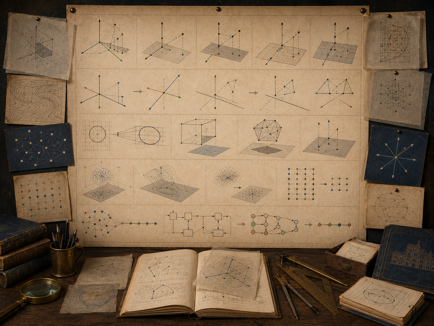
Projections and reflections are among the clearest examples of matrices as geometric actions. A projection sends a vector onto a subspace and leaves behind a residual. A reflection flips a vector across a line, plane, or subspace while preserving distance. Both operations reveal how linear algebra organizes space into meaningful directions.
For systems modeling, these ideas are not merely geometric exercises. Projection explains approximation, least squares, dimensional reduction, fitted values, residuals, and information loss. Reflection explains symmetry, sign reversal, invariance, coordinate transformation, and structure-preserving change. Together, they help connect algebraic computation to visual and interpretive understanding.
Why Geometric Interpretation Matters
Geometric interpretation matters because algebraic operations become easier to understand when their spatial behavior is visible. A matrix can be studied as an array, as a system of equations, as a transformation, or as an operation on geometry. Each view reveals something different.
For systems modeling, geometry helps answer practical questions. Which parts of the data are explained by a model? Which parts remain as residuals? Which directions are preserved? Which directions are reversed? Which components are removed? Which state differences are compressed? Which distances or angles matter?
| Geometric idea | Linear algebra role | Systems modeling interpretation |
|---|---|---|
| Projection | Maps vectors onto a subspace. | Approximation, fitted value, retained component, or simplified representation. |
| Residual | Difference between original vector and projection. | Unexplained variation, mismatch, error, or discarded information. |
| Reflection | Flips vectors across a subspace. | Symmetry, sign reversal, orientation change, or structure-preserving transformation. |
| Distance | Norm of a difference vector. | Magnitude of error, deviation, mismatch, or change. |
| Angle | Relationship between directions. | Alignment, opposition, independence, or correlation-like structure. |
Geometry turns abstract matrix action into interpretable model behavior.
Matrices as Geometric Actions
A matrix transforms space. Some transformations preserve length. Some preserve angles. Some collapse dimension. Some reverse orientation. Some keep one subspace fixed while changing another. Projection and reflection are especially useful because their geometric actions are precise and interpretable.
T(\mathbf{x})=A\mathbf{x}
\]
Interpretation: A matrix \(A\) acts on a vector \(\mathbf{x}\), producing a transformed state whose geometric behavior can be analyzed.
The transformation view makes it possible to describe matrices by what they do. A projection matrix asks: what part of the vector belongs to a chosen subspace? A reflection matrix asks: what happens when a vector is mirrored across a chosen geometric structure?
| Transformation | Geometric action | Modeling meaning |
|---|---|---|
| Projection | Moves vector onto a subspace. | Retains modeled structure and separates residuals. |
| Reflection | Flips vector across a line, plane, or subspace. | Tests symmetry, reverses orientation, or preserves distance while changing direction. |
| Rotation | Turns space around an origin. | Changes coordinate orientation while preserving distance. |
| Shear | Slants space while preserving parallel structure. | Models directional dependence or distortion. |
| Scaling | Expands or contracts directions. | Amplifies, dampens, or rescales components. |
| Collapse | Maps space into lower dimension. | Loses information or simplifies representation. |
Projection and reflection give a bridge between visual intuition and rigorous computation.
What Is a Projection?
A projection maps a vector onto a subspace. The projected vector is the component of the original vector that lies in the subspace. The difference between the original vector and the projection is the residual.
\mathbf{x}=\operatorname{proj}_{S}(\mathbf{x})+\mathbf{r}
\]
Interpretation: A vector can be decomposed into a projected component inside a subspace \(S\) and a residual component outside the represented structure.
Projection is the geometry behind approximation. When a model cannot exactly represent a vector, the projection finds the closest representable vector under the chosen distance measure. This is why projections are central to least squares, regression, signal approximation, dimensionality reduction, and model fitting.
| Projection element | Formal meaning | Systems modeling interpretation |
|---|---|---|
| Original vector | \(\mathbf{x}\) | Observed state, measured data, target vector, or full system signal. |
| Subspace | \(S\) | Model-representable structure or allowed pattern space. |
| Projection | \(\operatorname{proj}_{S}(\mathbf{x})\) | Fitted, simplified, retained, or modeled component. |
| Residual | \(\mathbf{r}=\mathbf{x}-\operatorname{proj}_{S}(\mathbf{x})\) | Unexplained, discarded, or unmodeled component. |
| Distance | \(\|\mathbf{r}\|\) | Approximation error or mismatch magnitude. |
Projection makes approximation geometrically explicit.
Orthogonal Projection onto a Vector
The simplest projection sends a vector \(\mathbf{x}\) onto the line spanned by a nonzero vector \(\mathbf{u}\). The result is the part of \(\mathbf{x}\) that points in the direction of \(\mathbf{u}\).
\operatorname{proj}_{\mathbf{u}}(\mathbf{x})
=
\frac{\mathbf{x}\cdot\mathbf{u}}{\mathbf{u}\cdot\mathbf{u}}\mathbf{u}
\]
Interpretation: The projection keeps the component of \(\mathbf{x}\) aligned with \(\mathbf{u}\) and removes the perpendicular part.
The scalar coefficient measures how much of the direction \(\mathbf{u}\) appears inside \(\mathbf{x}\). If the dot product is positive, the projection points with \(\mathbf{u}\). If it is negative, the projection points opposite \(\mathbf{u}\). If it is zero, the vectors are orthogonal and the projection is the zero vector.
| Dot-product case | Projection behavior | Modeling interpretation |
|---|---|---|
| \(\mathbf{x}\cdot\mathbf{u}>0\) | Projection points with \(\mathbf{u}\). | The state aligns with the modeled direction. |
| \(\mathbf{x}\cdot\mathbf{u}<0\) | Projection points opposite \(\mathbf{u}\). | The state opposes the modeled direction. |
| \(\mathbf{x}\cdot\mathbf{u}=0\) | Projection is zero. | The state has no component in that direction. |
| Large projected norm | Strong component along \(\mathbf{u}\). | The direction explains substantial structure. |
| Large residual norm | Weak representation by \(\mathbf{u}\). | The direction fails to capture important structure. |
Projection onto one vector is the foundation for projection onto larger subspaces.
Projection onto a Subspace
Many models approximate data using a subspace rather than a single direction. If the columns of \(A\) span a subspace, then projecting \(\mathbf{b}\) onto the column space of \(A\) finds the closest vector to \(\mathbf{b}\) that the model can represent.
\widehat{\mathbf{b}}\in\operatorname{Col}(A),\qquad
\mathbf{r}=\mathbf{b}-\widehat{\mathbf{b}}
\]
Interpretation: The projected vector \(\widehat{\mathbf{b}}\) is the model-representable component of \(\mathbf{b}\), and the residual \(\mathbf{r}\) is what remains outside the column space.
Projection onto a subspace is not merely a geometric convenience. It is the conceptual foundation of least-squares modeling. When a system of equations is inconsistent, the right-hand side does not lie in the column space. Least squares replaces the unreachable target with its closest reachable approximation.
| Subspace projection object | Formal role | Systems modeling interpretation |
|---|---|---|
| \(\operatorname{Col}(A)\) | Model-representable output space. | All outputs the linear model can produce. |
| \(\mathbf{b}\) | Observed or target vector. | Measurement, demand, signal, response, or empirical target. |
| \(\widehat{\mathbf{b}}\) | Projection of \(\mathbf{b}\) into \(\operatorname{Col}(A)\). | Fitted value or closest model-produced approximation. |
| \(\mathbf{r}\) | Residual vector. | Unexplained structure, mismatch, noise, or model limitation. |
| \(\|\mathbf{r}\|\) | Projection error distance. | Magnitude of model-target mismatch. |
Subspace projection gives linear models their geometry of approximation.
Projection Matrices
A projection matrix is a matrix \(P\) that projects vectors onto a subspace. For orthogonal projection onto the column space of a full-column-rank matrix \(A\), the projection matrix is:
P=A(A^TA)^{-1}A^T
\]
Interpretation: The projection matrix maps any vector onto the column space of \(A\), assuming \(A\) has full column rank.
A projection matrix has a defining property: applying it twice does nothing more than applying it once. Once a vector is already projected onto the subspace, projecting it again leaves it unchanged.
P^2=P
\]
Interpretation: Projection matrices are idempotent: once a vector has been projected, repeating the projection does not change it.
For orthogonal projection, the projection matrix is also symmetric:
P^T=P
\]
Interpretation: Symmetry means the projection is orthogonal under the standard inner product.
| Projection-matrix property | Formal meaning | Modeling interpretation |
|---|---|---|
| Idempotence | \(P^2=P\) | Once fitted, refitting to the same subspace changes nothing. |
| Symmetry | \(P^T=P\) | Projection is orthogonal under the chosen geometry. |
| Rank | \(\operatorname{rank}(P)=\dim(S)\) | Number of retained independent directions. |
| Eigenvalues | Usually \(0\) or \(1\) for orthogonal projection. | Directions are either retained or removed. |
| Residual operator | \(I-P\) | Maps vectors to their unmodeled component. |
Projection matrices make retention and residual structure explicit.
Residuals and Orthogonality
In orthogonal projection, the residual is perpendicular to the subspace. This is the geometric reason the projection is the closest point in the subspace.
A^T(\mathbf{b}-A\widehat{\mathbf{x}})=\mathbf{0}
\]
Interpretation: The residual is orthogonal to every column of \(A\), meaning no remaining residual component lies in the modeled directions.
This condition is more than a technical result. It explains why least squares works. The fitted component captures everything in the column-space directions. The residual is what cannot be explained by those directions.
| Residual condition | Geometric meaning | Systems modeling interpretation |
|---|---|---|
| \(\mathbf{r}=\mathbf{b}-\widehat{\mathbf{b}}\) | Difference between observed and fitted vector. | Unexplained or unmodeled component. |
| \(\mathbf{r}\perp\operatorname{Col}(A)\) | Residual is perpendicular to model space. | No model direction can further reduce the residual. |
| \(A^T\mathbf{r}=0\) | Normal equations condition. | Each model feature is orthogonal to the remaining error. |
| \(\|\mathbf{r}\|\) | Distance to the subspace. | Approximation error magnitude. |
| \(I-P\) | Residual projection operator. | Extracts what the model leaves out. |
Residuals are not leftovers to ignore. They are geometric evidence about what the model fails to represent.
Least-Squares Geometry
Least squares is projection geometry. When \(A\mathbf{x}=\mathbf{b}\) has no exact solution, the target \(\mathbf{b}\) lies outside the column space of \(A\). Least squares finds the vector \(A\widehat{\mathbf{x}}\) inside the column space that is closest to \(\mathbf{b}\).
\widehat{\mathbf{x}}=\arg\min_{\mathbf{x}}\|A\mathbf{x}-\mathbf{b}\|_2^2
\]
Interpretation: Least squares chooses the coefficient vector whose model-produced output is closest to the observed target.
The fitted vector is:
\widehat{\mathbf{b}}=A\widehat{\mathbf{x}}
\]
Interpretation: The fitted vector is the projection of \(\mathbf{b}\) onto the column space of \(A\).
This geometric view prevents a common mistake: treating least squares as if it “solves” an inconsistent system exactly. It does not. It finds the closest reachable approximation under a particular geometry and error criterion.
| Least-squares object | Projection interpretation | Modeling caution |
|---|---|---|
| \(A\) | Defines the model subspace. | Column meanings and scaling shape the approximation. |
| \(\mathbf{b}\) | Target vector outside or inside the subspace. | Measurements may include noise, bias, or incompatible structure. |
| \(\widehat{\mathbf{x}}\) | Coordinates of closest point in model space. | Coefficients are not automatically causal or stable. |
| \(\widehat{\mathbf{b}}\) | Projection of target onto column space. | Fitted value is model-representable approximation. |
| \(\mathbf{r}\) | Perpendicular error vector. | Residuals require interpretation, diagnostics, and review. |
Least-squares modeling is projection plus interpretation.
What Is a Reflection?
A reflection flips a vector across a line, plane, or subspace. Unlike projection, reflection does not usually discard information. It preserves distance while reversing the component perpendicular to the reflecting subspace.
For a reflection across a subspace \(S\), the component inside \(S\) is preserved, while the component perpendicular to \(S\) changes sign.
\mathbf{x}=\mathbf{x}_{S}+\mathbf{x}_{S^\perp}
\quad\Longrightarrow\quad
R\mathbf{x}=\mathbf{x}_{S}-\mathbf{x}_{S^\perp}
\]
Interpretation: Reflection preserves the component inside the mirror subspace and reverses the perpendicular component.
| Reflection component | Geometric behavior | Modeling interpretation |
|---|---|---|
| Component in mirror subspace | Preserved. | Structure aligned with the reference frame remains unchanged. |
| Perpendicular component | Sign is reversed. | Deviation from the reference structure is mirrored. |
| Distance from origin | Preserved. | Magnitude remains constant under reflection. |
| Angle structure | Preserved. | Reflection is a rigid transformation. |
| Orientation | Reversed in appropriate dimensions. | Coordinate handedness or directionality may flip. |
Reflection is a structure-preserving transformation with a reversal component.
Reflection Matrices
A reflection matrix can be built from a projection matrix. If \(P\) projects onto the mirror subspace, then the reflection across that subspace is:
R=2P-I
\]
Interpretation: Reflection doubles the projected component and subtracts the original vector, leaving the parallel part fixed and flipping the perpendicular part.
For reflection across a line spanned by a unit vector \(\mathbf{u}\), the projection matrix is \(P=\mathbf{u}\mathbf{u}^T\), and the reflection matrix is:
R=2\mathbf{u}\mathbf{u}^T-I
\]
Interpretation: A unit direction \(\mathbf{u}\) defines the mirror line; the reflection preserves that direction and reverses the perpendicular direction.
Reflection matrices are orthogonal when the reflection is Euclidean. They preserve length and angle:
R^TR=I
\]
Interpretation: Euclidean reflections preserve distances and angles even while reversing orientation.
| Reflection property | Formal meaning | Systems modeling interpretation |
|---|---|---|
| Orthogonality | \(R^TR=I\) | Distances and angles are preserved. |
| Involution | \(R^2=I\) | Reflecting twice returns the original state. |
| Preserved subspace | \(R\mathbf{x}=\mathbf{x}\) for \(\mathbf{x}\in S\) | Reference-aligned structure remains unchanged. |
| Reversed subspace | \(R\mathbf{x}=-\mathbf{x}\) for \(\mathbf{x}\in S^\perp\) | Deviation from the reference structure flips. |
| Determinant | Often \(-1\) for a single hyperplane reflection. | Orientation is reversed. |
Reflection matrices reveal symmetry, reversal, and invariance in linear systems.
Projections vs. Reflections
Projection and reflection are closely related but behaviorally different. Projection removes the perpendicular component. Reflection reverses it. Projection reduces information. Reflection preserves information while changing orientation.
| Feature | Projection | Reflection |
|---|---|---|
| Action on subspace component | Preserves it. | Preserves it. |
| Action on perpendicular component | Removes it. | Reverses it. |
| Information preservation | Generally loses information. | Preserves information. |
| Distance preservation | Does not generally preserve distance. | Preserves distance in Euclidean reflection. |
| Repeated application | \(P^2=P\) | \(R^2=I\) |
| Modeling meaning | Approximation and simplification. | Symmetry and reversal. |
This distinction matters in systems modeling. A projection may simplify a dataset by discarding residual structure. A reflection may test symmetry or change orientation without losing magnitude. Confusing the two can lead to incorrect interpretation.
Distance, Angle, and Structure
Geometric interpretation depends on distance and angle. Projections use distance to define closest approximation. Reflections preserve distance and angle while changing orientation. Both rely on an inner product, usually the standard dot product unless another geometry is specified.
\|\mathbf{x}-\widehat{\mathbf{x}}\|
\]
Interpretation: Distance measures how far an original vector is from its projected approximation.
\mathbf{u}\cdot\mathbf{v}=0
\]
Interpretation: Orthogonality means two directions are perpendicular under the chosen inner product.
The phrase “chosen inner product” matters. In many systems, the standard Euclidean geometry may not be the right geometry. Weighted least squares, covariance-based distances, energy norms, and domain-specific metrics can change what “closest,” “orthogonal,” or “residual” means.
| Geometric measure | Standard meaning | Modeling caution |
|---|---|---|
| Euclidean distance | Straight-line norm. | May ignore units, weights, uncertainty, or covariance. |
| Orthogonality | Zero dot product. | Depends on the chosen inner product. |
| Angle | Directional alignment. | Can be distorted by scaling or normalization. |
| Projection error | Residual norm. | Small residual does not guarantee valid interpretation. |
| Reflection symmetry | Mirror behavior. | May be a mathematical symmetry rather than a real-world mechanism. |
Geometry is powerful, but it must match the modeling context.
Geometric Interpretation in Systems Modeling
In systems modeling, projections help clarify approximation, filtering, model fit, retained structure, and residual structure. Reflections help clarify symmetry, reversibility, orientation, and invariance. Both operations support a larger skill: reading linear algebra as geometry.
Infrastructure systems may project high-dimensional condition data onto vulnerability modes. Economic systems may project sectoral activity onto dominant demand patterns. Ecological systems may project observations onto interaction gradients. Machine-learning pipelines may project features into lower-dimensional embeddings. Scientific workflows may use reflections inside stable numerical algorithms, including Householder transformations.
| Domain | Projection use | Reflection use |
|---|---|---|
| Infrastructure planning | Project asset data onto risk or service modes. | Test symmetric response assumptions or transform coordinate frames. |
| Economic modeling | Project activity onto sectoral or demand subspaces. | Analyze sign-reversal or symmetry in transformed representations. |
| Ecological modeling | Separate modeled gradients from residual variation. | Study mirrored deviations around equilibrium-like references. |
| Machine learning | Reduce dimension, fit features, or extract latent structure. | Use reflection-like transformations in stable algorithms. |
| Scientific computing | Use projections in least squares and decompositions. | Use Householder reflections for QR factorization. |
| Policy analysis | Project indicators into composite dimensions. | Examine how sign or orientation changes affect interpretation. |
Projection and reflection are not isolated techniques. They are building blocks of applied linear algebra.
Numerical Stability and Diagnostics
Geometric transformations should be audited numerically. A projection matrix computed through \((A^TA)^{-1}\) can be unstable when columns of \(A\) are nearly dependent. In serious scientific computing, QR or SVD-based methods are often more reliable than explicitly forming normal-equation inverses.
Projection workflows should check rank, condition number, residual norm, idempotence error, symmetry error, and reconstruction behavior. Reflection workflows should check orthogonality, involution error, length preservation, determinant when relevant, and orientation effects.
| Diagnostic | Projection relevance | Reflection relevance |
|---|---|---|
| Rank | Checks subspace dimension and dependence. | Checks basis or mirror-subspace construction. |
| Condition number | Flags unstable projection formulas. | Flags unstable basis construction. |
| Idempotence error | Checks whether \(P^2\approx P\). | Not primary. |
| Symmetry error | Checks whether projection is orthogonal. | Checks structure when reflection is built from projection. |
| Involution error | Not primary. | Checks whether \(R^2\approx I\). |
| Length preservation | Not generally expected. | Expected for Euclidean reflections. |
| Residual norm | Measures approximation error. | Can measure deviation from symmetry. |
Geometric interpretation should be paired with numerical checks, especially when projections or reflections support decisions.
Mathematical Deepening
This section adds a more formal layer for mathematically advanced readers. Projections and reflections connect subspaces, direct sums, orthogonal complements, inner products, normal equations, idempotent operators, symmetric operators, orthogonal transformations, invariant subspaces, least squares, QR factorization, Householder reflections, and numerical stability.
Projection Structure
Subspace
A projection is defined relative to a target subspace that represents retained structure.
Projected Component
The projected component lies in the target subspace and is the modeled or retained part.
Residual Component
The residual component lies outside the retained representation and measures mismatch.
Orthogonal Complement
For orthogonal projection, the residual belongs to the orthogonal complement of the target subspace.
Operator Properties
Idempotence
Projection satisfies \(P^2=P\), meaning repeated projection does not change the result.
Symmetry
Orthogonal projection satisfies \(P^T=P\) under the standard Euclidean inner product.
Involution
Reflection satisfies \(R^2=I\), meaning reflecting twice recovers the original vector.
Orthogonality
Euclidean reflection satisfies \(R^TR=I\), preserving lengths and angles.
Least Squares and Projection
Column Space
The column space of \(A\) is the set of model-representable outputs.
Normal Equations
The condition \(A^T(\mathbf{b}-A\widehat{\mathbf{x}})=0\) says the residual is orthogonal to the model space.
Projection Matrix
When full rank, \(P=A(A^TA)^{-1}A^T\) maps targets to fitted values.
Residual Operator
The matrix \(I-P\) extracts the component not explained by the model space.
Reflection Structure
Mirror Subspace
The subspace across which reflection preserves aligned components.
Perpendicular Reversal
The component perpendicular to the mirror subspace changes sign.
Householder Reflection
A reflection used in numerical algorithms to zero selected vector components stably.
Orientation
Reflection can preserve distances while reversing orientation.
Governance Questions
What Is Being Retained?
Projection requires a clear account of the subspace treated as meaningful structure.
What Is Being Discarded?
The residual may contain noise, bias, unmodeled mechanism, or important excluded structure.
What Geometry Is Used?
Distance, angle, and orthogonality depend on the chosen inner product or weighting.
Is the Computation Stable?
Projection and reflection workflows should include rank, conditioning, and operator-property checks.
Examples from Systems Modeling
Projections and reflections appear whenever a model separates retained structure from residual structure, or uses geometric transformation to preserve or reverse system features.
Infrastructure Risk Modes
Condition measurements can be projected onto vulnerability modes, separating dominant risk patterns from residual local variation.
Economic Sector Approximation
Sectoral activity can be projected onto a lower-dimensional production subspace, revealing fitted structure and unexplained demand patterns.
Ecological Gradient Modeling
Species observations can be projected onto environmental gradients, separating modeled ecological response from residual variation.
Machine Learning Feature Reduction
High-dimensional feature vectors can be projected into lower-dimensional spaces, improving compression while discarding some information.
Scientific Computing with Reflections
Householder reflections can transform matrices stably during QR factorization and least-squares workflows.
Policy Indicator Geometry
Composite indicators may project many measures into selected dimensions, requiring careful interpretation of what is retained and omitted.
Across these examples, the geometry should be documented as part of the modeling claim, not hidden as a technical preprocessing step.
Computation and Reproducible Workflows
Computational workflows for projections and reflections should document the original vector, target subspace, projection matrix, projected vector, residual vector, residual norm, idempotence error, symmetry error, reflection matrix, reflected vector, length-preservation error, involution error, rank checks, condition warnings, and interpretation notes.
The companion repository treats geometric interpretation as auditable systems modeling. Python, R, Julia, SQL, Haskell, C, C++, Fortran, Rust, Go, notebooks, schemas, generated outputs, Canvas artifacts, advanced reports, and calculators each support a different layer of reproducible projection and reflection analysis.
For this article, the computational examples focus on projection operators, residual diagnostics, reflection operators, length preservation, and model-governance records.
Python Workflow: Projection and Reflection Audit
The Python workflow below projects a vector onto a line, computes the residual, constructs a reflection across that line, and records diagnostic checks.
from __future__ import annotations

from dataclasses import asdict, dataclass
from pathlib import Path
import csv
import json
import math


Vector = list[float]
Matrix = list[list[float]]


@dataclass(frozen=True)
class ProjectionReflectionAudit:
    system_name: str
    original_vector: str
    unit_direction: str
    projected_vector: str
    residual_vector: str
    residual_norm: float
    reflected_vector: str
    projection_idempotence_error: float
    projection_symmetry_error: float
    reflection_involution_error: float
    length_preservation_error: float
    interpretation_warning: str


def dot(a: Vector, b: Vector) -> float:
    return sum(x * y for x, y in zip(a, b))


def norm2(v: Vector) -> float:
    return math.sqrt(dot(v, v))


def matvec(A: Matrix, x: Vector) -> Vector:
    return [dot(row, x) for row in A]


def matmul(A: Matrix, B: Matrix) -> Matrix:
    return [
        [sum(a * b for a, b in zip(row, col)) for col in zip(*B)]
        for row in A
    ]


def transpose(A: Matrix) -> Matrix:
    return [list(col) for col in zip(*A)]


def outer(u: Vector, v: Vector) -> Matrix:
    return [[a * b for b in v] for a in u]


def identity(n: int) -> Matrix:
    return [[1.0 if i == j else 0.0 for j in range(n)] for i in range(n)]


def matrix_subtract(A: Matrix, B: Matrix) -> Matrix:
    return [[a - b for a, b in zip(row_a, row_b)] for row_a, row_b in zip(A, B)]


def vector_subtract(a: Vector, b: Vector) -> Vector:
    return [x - y for x, y in zip(a, b)]


def matrix_norm(A: Matrix) -> float:
    return math.sqrt(sum(value * value for row in A for value in row))


def vector_to_string(v: Vector) -> str:
    return ",".join(f"{value:.6f}" for value in v)


def build_audit() -> ProjectionReflectionAudit:
    x = [4.0, 3.0]
    direction = [2.0, 1.0]
    direction_norm = norm2(direction)
    u = [value / direction_norm for value in direction]

    P = outer(u, u)
    projected = matvec(P, x)
    residual = vector_subtract(x, projected)

    I = identity(2)
    R = [[2.0 * P[i][j] - I[i][j] for j in range(2)] for i in range(2)]
    reflected = matvec(R, x)

    projection_idempotence_error = matrix_norm(matrix_subtract(matmul(P, P), P))
    projection_symmetry_error = matrix_norm(matrix_subtract(transpose(P), P))
    reflection_involution_error = matrix_norm(matrix_subtract(matmul(R, R), I))
    length_preservation_error = abs(norm2(reflected) - norm2(x))

    return ProjectionReflectionAudit(
        system_name="two_dimensional_geometric_transformation_audit",
        original_vector=vector_to_string(x),
        unit_direction=vector_to_string(u),
        projected_vector=vector_to_string(projected),
        residual_vector=vector_to_string(residual),
        residual_norm=round(norm2(residual), 12),
        reflected_vector=vector_to_string(reflected),
        projection_idempotence_error=round(projection_idempotence_error, 12),
        projection_symmetry_error=round(projection_symmetry_error, 12),
        reflection_involution_error=round(reflection_involution_error, 12),
        length_preservation_error=round(length_preservation_error, 12),
        interpretation_warning=(
            "Projection retains the modeled direction and discards the perpendicular residual; "
            "reflection preserves distance while reversing the perpendicular component. "
            "Interpretation depends on the chosen geometry, units, scaling, and model purpose."
        ),
    )


def write_outputs(output_dir: Path) -> None:
    (output_dir / "tables").mkdir(parents=True, exist_ok=True)
    (output_dir / "json").mkdir(parents=True, exist_ok=True)

    audit = build_audit()
    row = asdict(audit)

    with (output_dir / "tables" / "projection_reflection_audit.csv").open(
        "w", newline="", encoding="utf-8"
    ) as handle:
        writer = csv.DictWriter(handle, fieldnames=list(row.keys()))
        writer.writeheader()
        writer.writerow(row)

    (output_dir / "json" / "projection_reflection_audit.json").write_text(
        json.dumps(row, indent=2, sort_keys=True),
        encoding="utf-8",
    )


if __name__ == "__main__":
    write_outputs(Path("outputs"))
    print("Projection and reflection audit complete.")
This workflow treats projection and reflection as auditable geometric transformations. It records projected structure, residual structure, reflected state, operator diagnostics, and interpretation warnings.
R Workflow: Geometric Transformation Diagnostics
R can support projection and reflection diagnostics by computing projection matrices, residual vectors, reflection matrices, and operator checks.
x <- c(4, 3)
direction <- c(2, 1)
u <- direction / sqrt(sum(direction^2))

P <- u %*% t(u)
projected <- as.vector(P %*% x)
residual <- x - projected
residual_norm <- sqrt(sum(residual^2))

I <- diag(2)
R <- 2 * P - I
reflected <- as.vector(R %*% x)

projection_idempotence_error <- sqrt(sum((P %*% P - P)^2))
projection_symmetry_error <- sqrt(sum((t(P) - P)^2))
reflection_involution_error <- sqrt(sum((R %*% R - I)^2))
length_preservation_error <- abs(sqrt(sum(reflected^2)) - sqrt(sum(x^2)))

audit_record <- data.frame(
  system_name = "two_dimensional_geometric_transformation_audit",
  original_vector = paste(round(x, 6), collapse = ","),
  unit_direction = paste(round(u, 6), collapse = ","),
  projected_vector = paste(round(projected, 6), collapse = ","),
  residual_vector = paste(round(residual, 6), collapse = ","),
  residual_norm = residual_norm,
  reflected_vector = paste(round(reflected, 6), collapse = ","),
  projection_idempotence_error = projection_idempotence_error,
  projection_symmetry_error = projection_symmetry_error,
  reflection_involution_error = reflection_involution_error,
  length_preservation_error = length_preservation_error,
  interpretation_warning = paste(
    "Projection retains modeled structure and discards residual structure;",
    "reflection preserves distance while reversing perpendicular structure;",
    "interpretation depends on geometry, units, scaling, and model purpose."
  )
)

dir.create("outputs/tables", recursive = TRUE, showWarnings = FALSE)

write.csv(
  audit_record,
  "outputs/tables/r_projection_reflection_audit.csv",
  row.names = FALSE
)

print(audit_record)
This R workflow is useful when projections and reflections support least squares, residual diagnostics, geometric data analysis, scientific computing, or representation review.
Haskell Workflow: Typed Geometry Records
Haskell can represent projection and reflection diagnostics as a typed record with fields for projected vector, residual vector, reflected vector, and operator-property checks.
module Main where

data ProjectionReflectionAudit = ProjectionReflectionAudit
  { systemName :: String
  , originalVector :: String
  , unitDirection :: String
  , projectedVector :: String
  , residualVector :: String
  , residualNorm :: Double
  , reflectedVector :: String
  , projectionIdempotenceError :: Double
  , projectionSymmetryError :: Double
  , reflectionInvolutionError :: Double
  , lengthPreservationError :: Double
  , interpretationWarning :: String
  } deriving (Show)

buildAudit :: ProjectionReflectionAudit
buildAudit =
  ProjectionReflectionAudit
    "two_dimensional_geometric_transformation_audit"
    "4.000000,3.000000"
    "0.894427,0.447214"
    "4.400000,2.200000"
    "-0.400000,0.800000"
    0.894427
    "4.800000,1.400000"
    0.0
    0.0
    0.0
    0.0
    "Projection retains modeled structure and residualizes the perpendicular component; reflection preserves distance while reversing the perpendicular component."

main :: IO ()
main =
  print buildAudit
The typed workflow keeps geometric calculations attached to their interpretation, rather than treating projection and reflection as anonymous matrix operations.
SQL Workflow: Geometric Assumption Registry
SQL can document projection and reflection assumptions when geometric workflows support dashboards, model audits, scientific-computing pipelines, residual diagnostics, or institutional reports.
CREATE TABLE geometric_transformation_assumption_registry (
    assumption_key TEXT PRIMARY KEY,
    assumption_name TEXT NOT NULL,
    mathematical_role TEXT NOT NULL,
    systems_modeling_role TEXT NOT NULL,
    review_warning TEXT NOT NULL
);

INSERT INTO geometric_transformation_assumption_registry VALUES
(
  'projection',
  'Projection',
  'Maps a vector onto a target subspace.',
  'Retains model-representable structure and separates residual structure.',
  'The target subspace must be justified.'
);

INSERT INTO geometric_transformation_assumption_registry VALUES
(
  'residual',
  'Residual',
  'Difference between the original vector and its projection.',
  'Represents unexplained, discarded, or unmodeled structure.',
  'Residuals may contain important signal, not merely noise.'
);

INSERT INTO geometric_transformation_assumption_registry VALUES
(
  'orthogonality',
  'Orthogonality',
  'Perpendicularity under an inner product.',
  'Defines what it means for residuals to be independent of modeled directions.',
  'Orthogonality depends on the chosen geometry or weighting.'
);

INSERT INTO geometric_transformation_assumption_registry VALUES
(
  'projection_matrix',
  'Projection matrix',
  'A matrix satisfying idempotence, with symmetry for orthogonal projection.',
  'Maps observations to fitted or retained structure.',
  'Projection matrices should be checked for idempotence and symmetry.'
);

INSERT INTO geometric_transformation_assumption_registry VALUES
(
  'reflection',
  'Reflection',
  'Preserves mirror-subspace components and reverses perpendicular components.',
  'Represents symmetry, reversal, or orientation change.',
  'Reflection is not the same as approximation or information loss.'
);

INSERT INTO geometric_transformation_assumption_registry VALUES
(
  'distance_geometry',
  'Distance geometry',
  'Uses norms and inner products to measure closeness and angle.',
  'Determines what counts as closest approximation or residual size.',
  'Units, scaling, and weighting affect geometric conclusions.'
);

SELECT
    assumption_name,
    mathematical_role,
    systems_modeling_role,
    review_warning
FROM geometric_transformation_assumption_registry
ORDER BY assumption_key;
This registry keeps geometric interpretation tied to projection, residuals, orthogonality, reflection, distance, and responsible model interpretation.
GitHub Repository
The companion repository for this article is designed as a reproducible mathematical-modeling workspace. It supports projection and reflection audits, residual diagnostics, operator-property checks, geometric transformation reports, SQL governance tables, generated outputs, advanced mathematical audit reports, and reusable calculator scripts.
Complete Code Repository
Companion article folder with Python, R, Julia, SQL, Haskell, C, C++, Fortran, Rust, Go, notebooks, documentation, synthetic teaching data, generated outputs, schemas, Canvas-ready workflow artifacts, and reusable calculator scripts for projections, reflections, geometric interpretation, projection matrices, residual vectors, orthogonality, least-squares geometry, reflection matrices, distance preservation, operator diagnostics, model governance, and responsible mathematical modeling.
Interpretive Limits and Responsible Use
Geometric interpretation is powerful because it makes matrix behavior visible. It is limited because geometry depends on representation, scaling, units, distance choices, and modeling purpose. A projection may look like a clean approximation while discarding important structure. A residual may be treated as noise even when it contains excluded mechanism, bias, or domain-relevant signal. A reflection may represent elegant symmetry that the real system does not actually possess.
Projection workflows require special caution. Choosing a subspace is a modeling decision. Choosing a norm is a modeling decision. Choosing to minimize squared error is a modeling decision. The closest point in Euclidean geometry may not be the most meaningful approximation for a social, ecological, economic, infrastructural, or institutional system.
Responsible use requires documenting the target subspace, the chosen inner product, units, scaling, residual interpretation, projection diagnostics, reflection diagnostics, numerical method, conditioning, and whether the transformation is used for explanation, approximation, compression, prediction, simulation, or decision support.
Related Articles
- What Is Linear Algebra for Systems Modeling?
- Scalars, Vectors, and System States
- Vector Spaces and System Representation
- Span, Linear Independence, and Basis
- Dimension and the Structure of Solution Spaces
- Matrices and the Organization of Multivariable Systems
- Matrix Arithmetic and the Logic of Combination
- Systems of Linear Equations
- Gaussian Elimination and Row Reduction
- Pivot Structure and Solvability
- Rank, Nullity, and Structural Dependence
- Determinants and Invertibility
- Inverse Matrices and Structural Recovery
- Overdetermined Systems and Least Squares Thinking
- Linear Transformations and Model Behavior
- Matrix Multiplication and Interaction Effects
- Change of Basis and Alternative Representations
- Linear Algebra for Systems Modeling
- Mathematical Modeling
- Systems Modeling
- Scientific Computing for Systems Modeling
Further Reading
- Axler, S. (2024) Linear Algebra Done Right. 4th edn. Cham: Springer. Available at: https://linear.axler.net/.
- Boyd, S. and Vandenberghe, L. (2018) Introduction to Applied Linear Algebra: Vectors, Matrices, and Least Squares. Cambridge: Cambridge University Press. Available at: https://vmls-book.stanford.edu/.
- Boyd, S. and Vandenberghe, L. (2018) Introduction to Applied Linear Algebra: Vectors, Matrices, and Least Squares. PDF edition. Stanford University and UCLA. Available at: https://web.stanford.edu/~boyd/vmls/vmls.pdf.
- Georgia Institute of Technology (n.d.) Interactive Linear Algebra. Georgia Institute of Technology. Available at: https://textbooks.math.gatech.edu/ila/.
- Golub, G.H. and Van Loan, C.F. (2013) Matrix Computations. 4th edn. Baltimore, MD: Johns Hopkins University Press. Available at: https://www.press.jhu.edu/books/title/10678/matrix-computations.
- Hefferon, J. (n.d.) Linear Algebra. Saint Michael’s College. Available at: https://joshua.smcvt.edu/linearalgebra/.
- Higham, N.J. (2002) Accuracy and Stability of Numerical Algorithms. 2nd edn. Philadelphia, PA: Society for Industrial and Applied Mathematics. Available at: https://epubs.siam.org/doi/book/10.1137/1.9780898718027.
- Horn, R.A. and Johnson, C.R. (2013) Matrix Analysis. 2nd edn. Cambridge: Cambridge University Press. Available at: https://www.cambridge.org/highereducation/books/matrix-analysis/FDA3627DC2B9F5C3DF2FD8C3CC136B48.
- Julia Documentation (n.d.) Linear Algebra — Julia Standard Library. Julia Documentation. Available at: https://docs.julialang.org/en/v1/stdlib/LinearAlgebra/.
- Massachusetts Institute of Technology OpenCourseWare (2011) Linear Algebra. Cambridge, MA: MIT OpenCourseWare. Available at: https://ocw.mit.edu/courses/18-06sc-linear-algebra-fall-2011/.
- Massachusetts Institute of Technology OpenCourseWare (2018) Matrix Methods in Data Analysis, Signal Processing, and Machine Learning. Cambridge, MA: MIT OpenCourseWare. Available at: https://ocw.mit.edu/courses/18-065-matrix-methods-in-data-analysis-signal-processing-and-machine-learning-spring-2018/.
- Meyer, C.D. (2023) Matrix Analysis and Applied Linear Algebra. 2nd edn. Philadelphia, PA: Society for Industrial and Applied Mathematics. Available at: https://epubs.siam.org/doi/book/10.1137/1.9781611977448.
- MIT Mathematics (2023) Introduction to Linear Algebra, Sixth Edition. Cambridge, MA: Massachusetts Institute of Technology. Available at: https://math.mit.edu/~gs/linearalgebra/ila6/indexila6.html.
- National Institute of Standards and Technology (n.d.) Matrix Market. NIST Mathematical and Computational Sciences Division. Available at: https://math.nist.gov/MatrixMarket/.
- Netlib (n.d.) BLAS — Basic Linear Algebra Subprograms. Netlib Repository. Available at: https://www.netlib.org/blas/.
- Netlib (n.d.) LAPACK — Linear Algebra PACKage. Netlib Repository. Available at: https://www.netlib.org/lapack/.
- Netlib and SIAM (1999) LAPACK Users’ Guide. 3rd edn. Philadelphia, PA: Society for Industrial and Applied Mathematics. Available at: https://www.netlib.org/lapack/lug/.
- NumPy Developers (n.d.) Linear Algebra: numpy.linalg. NumPy Documentation. Available at: https://numpy.org/doc/stable/reference/routines.linalg.html.
- SciPy Developers (n.d.) Linear Algebra: scipy.linalg. SciPy Documentation. Available at: https://docs.scipy.org/doc/scipy/reference/linalg.html.
- Strang, G. (2016) Introduction to Linear Algebra. Wellesley, MA: Wellesley-Cambridge Press. Available at: https://math.mit.edu/~gs/linearalgebra/.
- Treil, S. (2017) Linear Algebra Done Wrong. Providence, RI: Brown University. Available at: https://www.math.brown.edu/streil/papers/LADW/LADW.html.
- Trefethen, L.N. and Bau, D. (1997) Numerical Linear Algebra. Philadelphia, PA: Society for Industrial and Applied Mathematics. Available at: https://epubs.siam.org/doi/book/10.1137/1.9780898719574.
- van de Geijn, R. and Myers, M. (n.d.) Linear Algebra: Foundations to Frontiers. Austin, TX: The University of Texas at Austin. Available at: https://www.cs.utexas.edu/~flame/laff/laff/LAFF-2.00M.pdf.
References
- Axler, S. (2024) Linear Algebra Done Right. 4th edn. Cham: Springer. Available at: https://linear.axler.net/.
- Boyd, S. and Vandenberghe, L. (2018) Introduction to Applied Linear Algebra: Vectors, Matrices, and Least Squares. Cambridge: Cambridge University Press. Available at: https://vmls-book.stanford.edu/.
- Georgia Institute of Technology (n.d.) Interactive Linear Algebra. Georgia Institute of Technology. Available at: https://textbooks.math.gatech.edu/ila/.
- Golub, G.H. and Van Loan, C.F. (2013) Matrix Computations. 4th edn. Baltimore, MD: Johns Hopkins University Press. Available at: https://www.press.jhu.edu/books/title/10678/matrix-computations.
- Hefferon, J. (n.d.) Linear Algebra. Saint Michael’s College. Available at: https://joshua.smcvt.edu/linearalgebra/.
- Higham, N.J. (2002) Accuracy and Stability of Numerical Algorithms. 2nd edn. Philadelphia, PA: Society for Industrial and Applied Mathematics. Available at: https://epubs.siam.org/doi/book/10.1137/1.9780898718027.
- Horn, R.A. and Johnson, C.R. (2013) Matrix Analysis. 2nd edn. Cambridge: Cambridge University Press. Available at: https://www.cambridge.org/highereducation/books/matrix-analysis/FDA3627DC2B9F5C3DF2FD8C3CC136B48.
- Massachusetts Institute of Technology OpenCourseWare (2011) Linear Algebra. Cambridge, MA: MIT OpenCourseWare. Available at: https://ocw.mit.edu/courses/18-06sc-linear-algebra-fall-2011/.
- Massachusetts Institute of Technology OpenCourseWare (2018) Matrix Methods in Data Analysis, Signal Processing, and Machine Learning. Cambridge, MA: MIT OpenCourseWare. Available at: https://ocw.mit.edu/courses/18-065-matrix-methods-in-data-analysis-signal-processing-and-machine-learning-spring-2018/.
- Meyer, C.D. (2023) Matrix Analysis and Applied Linear Algebra. 2nd edn. Philadelphia, PA: Society for Industrial and Applied Mathematics. Available at: https://epubs.siam.org/doi/book/10.1137/1.9781611977448.
- MIT Mathematics (2023) Introduction to Linear Algebra, Sixth Edition. Cambridge, MA: Massachusetts Institute of Technology. Available at: https://math.mit.edu/~gs/linearalgebra/ila6/indexila6.html.
- Netlib (n.d.) BLAS — Basic Linear Algebra Subprograms. Netlib Repository. Available at: https://www.netlib.org/blas/.
- Netlib (n.d.) LAPACK — Linear Algebra PACKage. Netlib Repository. Available at: https://www.netlib.org/lapack/.
- NumPy Developers (n.d.) Linear Algebra: numpy.linalg. NumPy Documentation. Available at: https://numpy.org/doc/stable/reference/routines.linalg.html.
- R Core Team and Matrix Package Authors (n.d.) Matrix: Sparse and Dense Matrix Classes and Methods. CRAN. Available at: https://cran.r-project.org/package=Matrix.
- SciPy Developers (n.d.) Linear Algebra: scipy.linalg. SciPy Documentation. Available at: https://docs.scipy.org/doc/scipy/reference/linalg.html.
- Strang, G. (2016) Introduction to Linear Algebra. Wellesley, MA: Wellesley-Cambridge Press. Available at: https://math.mit.edu/~gs/linearalgebra/.
- Treil, S. (2017) Linear Algebra Done Wrong. Providence, RI: Brown University. Available at: https://www.math.brown.edu/streil/papers/LADW/LADW.html.
- Trefethen, L.N. and Bau, D. (1997) Numerical Linear Algebra. Philadelphia, PA: Society for Industrial and Applied Mathematics. Available at: https://epubs.siam.org/doi/book/10.1137/1.9780898719574.
- van de Geijn, R. and Myers, M. (n.d.) Linear Algebra: Foundations to Frontiers. Austin, TX: The University of Texas at Austin. Available at: https://www.cs.utexas.edu/~flame/laff/laff/LAFF-2.00M.pdf.