
Last Updated June 29, 2026
Stability analysis with eigenvalues explains how linear algebra detects whether system modes decay, persist, oscillate, or amplify over time. When a system evolves through repeated transformation, its future behavior is shaped by the eigenvalues of the matrix that governs the update. Eigenvalues reveal whether perturbations fade, grow, reverse, cycle, or remain near equilibrium.
This article introduces stability analysis as a systems modeling workflow. It connects eigenvalues, eigenvectors, spectral radius, stable modes, unstable modes, marginal modes, equilibrium behavior, discrete-time dynamics, continuous-time dynamics, linearization, perturbations, oscillation, decay, amplification, numerical conditioning, and responsible interpretation.
The central modeling question is not only “Are the eigenvalues less than one?” It is “What kind of stability claim is justified by this model, this matrix, this time scale, and this interpretation of system behavior?”
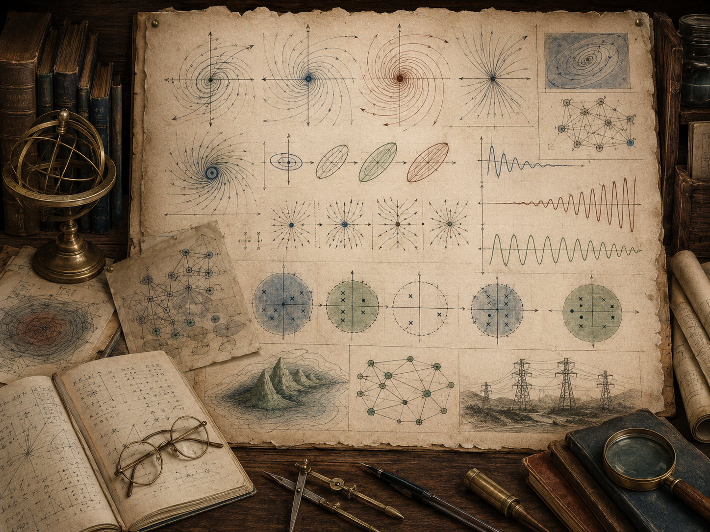
Stability is one of the most important ideas in systems modeling. A stable system can absorb small disturbances and return toward a reference state, equilibrium, trajectory, or acceptable operating region. An unstable system can amplify disturbances, drift away, oscillate dangerously, or enter regimes where the model no longer provides reliable guidance.
Eigenvalues provide a compact way to analyze stability in linear systems and local linear approximations. In discrete time, eigenvalue magnitude determines whether modes shrink or grow under repeated matrix application. In continuous time, eigenvalue real parts determine whether modes decay or amplify under exponential evolution. These rules are powerful, but they depend on modeling assumptions, scaling, time step, linearization, numerical conditioning, and domain interpretation.
Why Stability Analysis Matters
Stability analysis matters because systems are rarely observed only once. Infrastructure networks experience repeated stresses. Ecological populations evolve across seasons. Economic systems adjust over time. Algorithms iterate. Markov chains transition. Control systems respond to inputs. Scientific simulations advance through time steps. In each case, the modeler needs to know whether the system’s modes are damped, persistent, oscillatory, or amplifying.
Eigenvalues help answer that question. They identify how the natural modes of a linear system behave under repeated transformation or continuous evolution. Stability analysis turns eigenstructure into a judgment about system response.
| Stability question | Eigenvalue role | Systems modeling interpretation |
|---|---|---|
| Do disturbances fade? | Eigenvalues indicate decay. | The system may return toward equilibrium or baseline. |
| Do disturbances grow? | Eigenvalues indicate amplification. | The system may become unstable or sensitive to shocks. |
| Do modes persist? | Eigenvalues near stability boundary indicate slow or marginal behavior. | The system may have memory, inertia, conservation, or weak damping. |
| Do modes oscillate? | Complex eigenvalues indicate rotation or cycling. | The system may show cycles, waves, or alternating behavior. |
| Can the model support decisions? | Eigenvalue diagnostics support stability claims. | Results must be checked against assumptions and domain meaning. |
Stability analysis is not just a mathematical test. It is a structured way to ask whether modeled behavior remains bounded, meaningful, and usable over time.
Stability as System Behavior
In systems modeling, stability means more than “nothing changes.” A stable system can move, respond, fluctuate, and recover. Stability concerns how a system behaves after disturbance, whether it remains near a reference state, and whether errors or perturbations are damped rather than amplified.
Different fields use different stability concepts: asymptotic stability, Lyapunov stability, bounded-input bounded-output stability, marginal stability, numerical stability, structural stability, and practical stability. Eigenvalues are most directly tied to linear stability and local stability analysis.
| Stability concept | Basic idea | Modeling interpretation |
|---|---|---|
| Asymptotic stability | Disturbances decay over time. | The system returns toward equilibrium or reference behavior. |
| Marginal stability | Disturbances remain bounded but may not decay. | The system may persist, cycle, or conserve some mode. |
| Instability | Disturbances amplify. | Small deviations can become large or system-changing. |
| Local stability | Behavior near an equilibrium is stable. | A linearized model is useful only near the reference state. |
| Practical stability | Behavior remains within acceptable bounds. | Decision relevance depends on thresholds and consequences. |
Eigenvalues provide formal stability signals, but those signals must be interpreted in relation to the model’s purpose and the system’s operating context.
Linear Systems and Perturbations
A common stability question begins with a system near a reference state. The modeler asks what happens to a small perturbation. Does it shrink, persist, or grow?
In discrete time, a linear perturbation model can be written as:
\mathbf{x}_{t+1}=A\mathbf{x}_t
\]
Interpretation: The perturbation or state evolves by repeated application of the matrix \(A\).
In continuous time, a linear perturbation model can be written as:
\frac{d\mathbf{x}}{dt}=A\mathbf{x}
\]
Interpretation: The state changes continuously according to the matrix \(A\).
In both cases, eigenvalues describe modal behavior. The stability rule differs between discrete and continuous time, but the intuition is similar: some modes decay, some persist, and some amplify.
| Model type | State equation | Eigenvalue stability signal |
|---|---|---|
| Discrete time | \(\mathbf{x}_{t+1}=A\mathbf{x}_t\) | Eigenvalue magnitudes relative to \(1\). |
| Continuous time | \(\frac{d\mathbf{x}}{dt}=A\mathbf{x}\) | Eigenvalue real parts relative to \(0\). |
| Linearized nonlinear system | \(\Delta\mathbf{x}_{t+1}\approx J\Delta\mathbf{x}_t\) or \(\frac{d\Delta\mathbf{x}}{dt}\approx J\Delta\mathbf{x}\) | Eigenvalues of the Jacobian matrix near equilibrium. |
| Iterative algorithm | \(\mathbf{e}_{k+1}=A\mathbf{e}_k\) | Error modes decay or amplify depending on eigenvalues. |
| Transition process | \(\mathbf{p}_{t+1}=P\mathbf{p}_t\) | Eigenvalues affect convergence and long-run distribution. |
Stability analysis begins by clarifying the system equation, time model, and interpretation of the state vector.
Discrete-Time Stability
For a discrete-time linear system, repeated behavior is governed by powers of the matrix:
\mathbf{x}_t=A^t\mathbf{x}_0
\]
Interpretation: The state after \(t\) steps depends on the initial state and repeated matrix application.
If the matrix can be diagonalized, each mode evolves by powers of its eigenvalue:
A^t=P D^t P^{-1},
\qquad
D^t=\operatorname{diag}(\lambda_1^t,\lambda_2^t,\ldots,\lambda_n^t)
\]
Interpretation: Each mode grows, decays, persists, or alternates according to powers of its eigenvalue.
In discrete time, the key threshold is the unit circle. A mode decays if its eigenvalue magnitude is less than one. It grows if the magnitude is greater than one. It may persist or oscillate if the magnitude is exactly one.
| Discrete-time eigenvalue case | Mode behavior | Systems modeling interpretation |
|---|---|---|
| \(|\lambda|<1\) | \(\lambda^t\to0\) | Mode decays over repeated steps. |
| \(|\lambda|>1\) | Magnitude grows. | Mode amplifies or destabilizes. |
| \(\lambda=1\) | Mode persists. | Steady, conserved, or persistent component. |
| \(\lambda=-1\) | Mode alternates sign. | Repeated reversal without decay. |
| \(|\lambda|=1\), complex | Oscillation or rotation. | Persistent cycle may occur. |
For discrete-time stability, eigenvalue magnitudes determine whether modes are inside, outside, or on the unit circle.
Spectral Radius
The spectral radius of a matrix is the largest magnitude among its eigenvalues:
\rho(A)=\max_i|\lambda_i|
\]
Interpretation: The spectral radius identifies the largest modal amplification factor in a discrete-time system.
For many discrete-time linear systems, the spectral radius determines asymptotic stability. If \(\rho(A)<1\), all eigenvalue magnitudes are less than one, so modal components tend to decay under repeated application. If \(\rho(A)>1\), at least one mode amplifies.
| Spectral radius | Discrete-time implication | Modeling interpretation |
|---|---|---|
| \(\rho(A)<1\) | All eigenvalue magnitudes are inside the unit circle. | The homogeneous linear system is asymptotically stable under standard assumptions. |
| \(\rho(A)=1\) | At least one mode lies on the stability boundary. | The system may be marginal, persistent, cyclic, or sensitive to structure. |
| \(\rho(A)>1\) | At least one mode lies outside the unit circle. | The system has an amplifying mode. |
| \(\rho(A)\) close to \(1\) | Slow decay or slow growth may occur. | Long memory, near-instability, or slow convergence may matter. |
| Large spectral gap | Dominant mode may be clearly separated. | Long-run behavior may be easier to interpret. |
The spectral radius is compact, but it should not be the only diagnostic. Nonnormality, conditioning, forcing, nonlinearities, and constraints can change the practical stability story.
Stable, Unstable, and Marginal Modes
Eigenvalues classify modes. A stable mode decays. An unstable mode grows. A marginal mode remains on a boundary where behavior may persist, oscillate, or require additional analysis.
For a diagonalized discrete-time system, each modal coordinate follows:
z_{i,t}=\lambda_i^t z_{i,0}
\]
Interpretation: The \(i\)-th modal coordinate evolves by powers of its eigenvalue.
| Mode class | Discrete-time condition | Behavior | Interpretive caution |
|---|---|---|---|
| Stable mode | \(|\lambda_i|<1\) | Decays over time. | Decay rate may be slow if \(|\lambda_i|\) is close to one. |
| Unstable mode | \(|\lambda_i|>1\) | Amplifies over time. | Amplification may push the system outside the linear model’s validity. |
| Persistent mode | \(\lambda_i=1\) | Remains unchanged. | May reflect conservation, equilibrium, or modeling artifact. |
| Alternating mode | \(\lambda_i<0\) | Changes sign each step. | Can create overshoot or period-two behavior. |
| Oscillatory mode | Complex eigenvalue | Cycles or rotates. | Magnitude determines damping or amplification. |
Mode classification helps translate eigenvalues into behavior, but classification alone does not explain why the system behaves that way.
Continuous-Time Stability
In continuous time, stability is governed by exponential behavior. For the linear system:
\frac{d\mathbf{x}}{dt}=A\mathbf{x}
\]
Interpretation: The state evolves continuously according to the matrix \(A\).
If \(A\) has an eigenvalue \(\lambda\), a corresponding mode evolves like:
e^{\lambda t}
\]
Interpretation: Continuous-time modal behavior depends on the exponential of the eigenvalue times time.
For continuous-time stability, the key threshold is the imaginary axis. The real part of each eigenvalue determines whether the corresponding mode decays or grows.
| Continuous-time eigenvalue case | Mode behavior | Systems modeling interpretation |
|---|---|---|
| \(\operatorname{Re}(\lambda)<0\) | Mode decays exponentially. | Stable damping around the reference state. |
| \(\operatorname{Re}(\lambda)>0\) | Mode grows exponentially. | Instability or amplification. |
| \(\operatorname{Re}(\lambda)=0\) | Boundary behavior. | Persistence, oscillation, or marginal dynamics may require deeper analysis. |
| Complex pair with negative real part | Damped oscillation. | Cyclic behavior fades over time. |
| Complex pair with positive real part | Growing oscillation. | Cyclic instability may amplify. |
Discrete-time and continuous-time stability use different thresholds. In discrete time, compare eigenvalue magnitudes to one. In continuous time, compare eigenvalue real parts to zero.
Real and Complex Eigenvalues
Real eigenvalues produce direct growth, decay, reversal, or persistence. Complex eigenvalues combine scaling with rotation. In real matrices, complex eigenvalues appear in conjugate pairs, producing real oscillatory behavior when paired together.
\lambda=a+bi
\]
Interpretation: The real part \(a\) controls growth or decay in continuous time, while the imaginary part \(b\) contributes oscillation.
In discrete time, a complex eigenvalue can be represented by magnitude and angle:
\lambda=re^{i\theta}
\]
Interpretation: The magnitude \(r\) controls growth or decay per step, while \(\theta\) controls rotation or phase.
| Eigenvalue type | Discrete-time interpretation | Continuous-time interpretation |
|---|---|---|
| Positive real | Growth or decay without sign reversal. | Exponential growth or decay depending on sign. |
| Negative real | Alternating sign with growth or decay. | Real negative eigenvalue produces exponential decay. |
| Complex with magnitude less than one | Damped oscillation. | Not the continuous-time criterion by itself. |
| Complex with negative real part | Not the discrete-time criterion by itself. | Damped oscillation. |
| Purely imaginary | Depends on magnitude in discrete time. | Boundary oscillation in continuous time. |
Complex eigenvalues are not exotic edge cases. They are common in systems with rotation, feedback, delay-like effects, cycles, waves, or coupled exchange.
Oscillation, Damping, and Amplification
Oscillation occurs when modes rotate or alternate rather than simply moving directly toward or away from equilibrium. Damping means the oscillation shrinks. Amplification means the oscillation grows. Eigenvalues identify these patterns when the system is linear or locally linearized.
| Behavior | Eigenvalue signal | System interpretation |
|---|---|---|
| Monotone decay | Positive real eigenvalue inside discrete unit circle or negative real continuous-time eigenvalue. | State moves toward equilibrium without oscillation. |
| Alternating decay | Negative discrete-time eigenvalue with magnitude below one. | State overshoots and reverses while shrinking. |
| Damped oscillation | Complex mode with stable magnitude or negative real part, depending on time model. | Cyclic behavior fades over time. |
| Persistent oscillation | Boundary eigenvalues. | Cycles may remain without damping under ideal assumptions. |
| Growing oscillation | Unstable complex mode. | Cyclic instability amplifies over time. |
Oscillation can be beneficial, harmless, or dangerous depending on the system. A damped control response may be acceptable. A growing oscillation in infrastructure, finance, ecology, or operations may signal risk.
Equilibrium and Local Linearization
Many real systems are nonlinear. Eigenvalue stability analysis often enters through local linearization around an equilibrium. If a nonlinear discrete-time system is:
\mathbf{x}_{t+1}=F(\mathbf{x}_t)
\]
Interpretation: The next state is produced by a nonlinear update rule.
An equilibrium \(\mathbf{x}^\ast\) satisfies:
F(\mathbf{x}^\ast)=\mathbf{x}^\ast
\]
Interpretation: At equilibrium, applying the update rule leaves the state unchanged.
Near the equilibrium, the system can be approximated by the Jacobian matrix:
\Delta\mathbf{x}_{t+1}\approx J(\mathbf{x}^\ast)\Delta\mathbf{x}_t
\]
Interpretation: Small deviations from equilibrium evolve approximately according to the Jacobian matrix.
Eigenvalues of the Jacobian describe local stability. This does not automatically prove global stability. The approximation may only be valid near the equilibrium.
| Step | Mathematical role | Modeling caution |
|---|---|---|
| Find equilibrium | Solve \(F(\mathbf{x}^\ast)=\mathbf{x}^\ast\) or \(f(\mathbf{x}^\ast)=0\). | There may be multiple equilibria. |
| Compute Jacobian | Linear approximation near equilibrium. | Derivative estimates may be uncertain. |
| Analyze eigenvalues | Classify local modes. | Eigenvalues describe local linear behavior. |
| Check nonlinear validity | Test whether local claims generalize. | Large deviations may behave differently. |
| Interpret in domain | Translate modes into system behavior. | Mathematical stability may not equal practical safety. |
Local linearization is powerful, but the word “local” should remain visible in every interpretation.
Diagonalization and Mode Separation
Diagonalization helps stability analysis by separating a system into independent modes. If \(A=PDP^{-1}\), then the dynamics can be rewritten in modal coordinates. Each modal component is governed by its eigenvalue.
\mathbf{z}_{t+1}=D\mathbf{z}_t
\]
Interpretation: In modal coordinates, a diagonalized discrete-time system evolves mode by mode.
This separation clarifies stability because each mode can be classified individually. However, diagonalization must be used carefully. If the eigenvector matrix \(P\) is ill-conditioned, modal coordinates may be numerically unstable. If the matrix is not diagonalizable, generalized modes or other decompositions may be required.
| Diagonalization feature | Stability benefit | Caution |
|---|---|---|
| Independent modes | Each eigenvalue controls one mode. | Modes may be abstract or hard to interpret. |
| Matrix powers | Repeated behavior becomes easier to analyze. | Initial conditions determine modal amplitudes. |
| Dominant mode | Largest eigenvalue magnitude may control long-run behavior. | Spectral gaps and conditioning matter. |
| Eigenvector basis | Allows modal coordinates. | Ill-conditioned bases produce fragile decompositions. |
| Failure to diagonalize | Signals more complicated modal structure. | Do not force a diagonal interpretation. |
Diagonalization is a tool for stability explanation, but it is not required for every stability result and not always numerically reliable.
Nonnormality and Transient Growth
Eigenvalues describe asymptotic behavior, but they may not fully describe short-run behavior. In nonnormal matrices, eigenvectors are not orthogonal, and transient growth can occur even when all eigenvalues suggest eventual decay.
This matters in systems where short-run amplification is consequential. A system may be asymptotically stable but still experience dangerous temporary growth after a disturbance.
A^TA\neq AA^T
\]
Interpretation: A real matrix is nonnormal when it does not commute with its transpose, which can make eigenvalue-only stability stories incomplete.
| Issue | Eigenvalue story | Additional concern |
|---|---|---|
| Asymptotic stability | All modes eventually decay. | Short-run amplification may still occur. |
| Nonnormality | Eigenvalues may look safe. | Eigenvectors may interact in ways that amplify transients. |
| Ill-conditioned eigenvectors | Modes may be mathematically present. | Small perturbations can change modal coordinates substantially. |
| Near stability boundary | Modes decay slowly. | Practical stability may be weak. |
| Forced system | Homogeneous modes may decay. | External inputs can sustain or amplify response. |
Responsible stability analysis should distinguish asymptotic decay from practical short-run safety.
Numerical Conditioning and Stability Diagnostics
Eigenvalue stability analysis depends on numerical computation. Matrices with clustered eigenvalues, repeated eigenvalues, poor scaling, high condition numbers, or nonnormal structure can produce fragile stability conclusions.
Useful diagnostics include eigenpair residuals, spectral radius, spectral gap, condition number, scaling review, matrix norm, reconstruction error, and perturbation sensitivity.
\|A\mathbf{v}-\lambda\mathbf{v}\|
\]
Interpretation: The eigenpair residual checks how well a computed eigenvalue and eigenvector satisfy the eigenvalue equation.
\operatorname{gap}(\lambda_i)=\min_{j\neq i}|\lambda_i-\lambda_j|
\]
Interpretation: A small spectral gap means nearby eigenvalues may make modes harder to distinguish robustly.
| Diagnostic | Purpose | Interpretive warning |
|---|---|---|
| Spectral radius | Checks largest discrete-time eigenvalue magnitude. | Useful for asymptotic stability, not the whole story. |
| Eigenpair residual | Checks computed eigenpairs. | Small residual does not prove domain meaning. |
| Spectral gap | Checks mode separation. | Small gaps can make dominant modes unstable to perturbation. |
| Conditioning | Assesses sensitivity. | Fragile eigenvectors can undermine interpretation. |
| Scaling review | Checks units and coordinate magnitudes. | Poor scaling can distort computed stability properties. |
| Perturbation test | Tests stability under small data changes. | Robust conclusions should survive plausible perturbations. |
Numerical stability diagnostics should be part of the workflow, not an afterthought added only when results look suspicious.
Stability in Systems Modeling
Stability analysis with eigenvalues appears in many systems contexts. It can describe whether a population model approaches a stable distribution, whether an infrastructure stress mode grows, whether an economic adjustment process converges, whether a numerical method dampens error, or whether a control system returns toward a desired state.
But the same eigenvalue rule can mean different things across domains. A stable ecological equilibrium may still be undesirable. A stable economic pattern may preserve inequality. A stable infrastructure operating point may be fragile under unmodeled shocks. A numerically stable workflow may still be substantively wrong.
| Domain | Stability use | Interpretive caution |
|---|---|---|
| Infrastructure systems | Identify amplifying vulnerability modes. | Physical constraints and cascading effects may be nonlinear. |
| Ecological systems | Analyze population equilibrium and disturbance response. | Thresholds, seasonality, and nonlinear feedback may dominate. |
| Economic systems | Study convergence, persistence, and amplification across sectors. | Stability does not imply fairness, welfare, or resilience. |
| Control systems | Assess response to perturbations and feedback design. | Inputs, outputs, observability, and controllability also matter. |
| Markov systems | Study convergence toward steady-state distributions. | Transition assumptions, reducibility, and periodicity matter. |
| Scientific computing | Assess error propagation and numerical reliability. | Floating-point precision, time step, and conditioning matter. |
Stability is a mathematical property and a modeling judgment. Both dimensions should be visible.
Mathematical Deepening
This section adds a more formal layer. Stability analysis with eigenvalues connects spectral radius, matrix powers, diagonalization, Jordan structure, Schur decomposition, Lyapunov stability, local linearization, Jacobian matrices, continuous-time semigroups, matrix exponentials, perturbation theory, nonnormality, pseudospectra, numerical conditioning, and control theory.
Discrete-Time Review
Unit Circle
Discrete-time stability compares eigenvalue magnitudes to one.
Spectral Radius
The largest eigenvalue magnitude often controls asymptotic behavior.
Matrix Powers
Repeated system behavior is governed by \(A^t\).
Modal Decay
Modes with \(|\lambda|<1\) decay under repeated application.
Continuous-Time Review
Imaginary Axis
Continuous-time stability compares eigenvalue real parts to zero.
Matrix Exponential
Continuous-time solutions involve \(e^{At}\).
Exponential Decay
Modes with negative real parts decay.
Exponential Growth
Modes with positive real parts amplify.
Local Stability Review
Equilibrium
An equilibrium is a state that remains unchanged under the system rule.
Jacobian
The Jacobian gives the local linear approximation near equilibrium.
Local Claim
Eigenvalues of the Jacobian support local stability claims.
Nonlinear Limits
Local stability does not automatically imply global system behavior.
Numerical Review
Eigenpair Residuals
Check \(\|A\mathbf{v}-\lambda\mathbf{v}\|\) for computed eigenpairs.
Spectral Gap
Review whether modes are clearly separated.
Nonnormality
Check whether transient growth may undermine eigenvalue-only interpretation.
Perturbation Sensitivity
Test whether stability classification survives plausible data changes.
Governance Questions
What Is Stable?
Define whether stability refers to equilibrium, trajectory, distribution, operating range, or decision threshold.
Stable for Whom?
A stable system can preserve harmful, inequitable, or fragile arrangements.
Stable Under What?
Identify disturbance size, time scale, forcing terms, and operating conditions.
Stable According to Which Model?
Eigenvalue stability depends on the matrix, scaling, linearization, and assumptions.
Examples from Systems Modeling
Stability analysis with eigenvalues appears whenever system behavior evolves over time and the modeler needs to know whether perturbations decay, persist, oscillate, or amplify.
Infrastructure Stress Modes
An infrastructure interaction matrix may reveal whether stress perturbations fade locally or amplify into cascading vulnerability.
Ecological Population Models
Eigenvalues of transition or Jacobian matrices can classify local stability around population equilibria.
Economic Adjustment Dynamics
Sector interaction matrices can show whether shocks decay, persist, or amplify across economic structure.
Control System Response
Eigenvalues help assess whether feedback moves a system toward a desired state or produces overshoot and instability.
Markov Chain Convergence
Eigenvalue structure influences whether a transition system converges toward a steady distribution and how quickly it mixes.
Numerical Error Propagation
Eigenvalues of iteration matrices can show whether computational errors are damped or amplified by repeated steps.
Across these examples, eigenvalues support stability claims only when the matrix, time scale, and system interpretation are defensible.
Computation and Reproducible Workflows
Computational workflows for stability analysis should document the matrix, time model, eigenvalues, spectral radius, continuous-time real parts, stability classification, dominant modes, spectral gaps, eigenpair residuals, scaling assumptions, perturbation tests, and interpretation warnings.
The companion repository treats eigenvalue stability analysis as auditable systems modeling. Python, R, Julia, SQL, Haskell, C, C++, Fortran, Rust, Go, notebooks, schemas, generated outputs, Canvas artifacts, advanced reports, and calculators each support a different layer of reproducible stability analysis.
For this article, the computational examples focus on discrete-time stability classification, continuous-time stability classification, spectral-radius review, real-part review, perturbation warnings, and model-governance records.
Python Workflow: Eigenvalue Stability Audit
The Python workflow below computes eigenvalue-based stability diagnostics for a two-mode teaching example. It reports discrete-time spectral radius, continuous-time real-part checks, and interpretation warnings.
from __future__ import annotations

from dataclasses import asdict, dataclass
from pathlib import Path
import csv
import json
import math


Matrix2 = list[list[float]]


@dataclass(frozen=True)
class StabilityAudit:
    system_name: str
    matrix_entries: str
    trace: float
    determinant: float
    eigenvalue_1: float
    eigenvalue_2: float
    spectral_radius: float
    discrete_time_classification: str
    continuous_time_real_part_classification: str
    dominant_mode_warning: str
    interpretation_warning: str


def trace_2x2(A: Matrix2) -> float:
    return A[0][0] + A[1][1]


def determinant_2x2(A: Matrix2) -> float:
    return A[0][0] * A[1][1] - A[0][1] * A[1][0]


def eigenvalues_2x2(A: Matrix2) -> tuple[float, float]:
    tr = trace_2x2(A)
    det = determinant_2x2(A)
    discriminant = tr * tr - 4.0 * det
    if discriminant < 0:
        raise ValueError("This teaching routine handles real eigenvalues only.")
    root = math.sqrt(discriminant)
    return ((tr + root) / 2.0, (tr - root) / 2.0)


def matrix_to_string(A: Matrix2) -> str:
    return ";".join(",".join(f"{value:.6f}" for value in row) for row in A)


def classify_discrete(eigenvalues: tuple[float, float]) -> str:
    spectral_radius = max(abs(value) for value in eigenvalues)
    if spectral_radius < 1.0:
        return "asymptotically_stable_discrete_time"
    if abs(spectral_radius - 1.0) <= 1e-10:
        return "boundary_or_marginal_discrete_time"
    return "unstable_discrete_time"


def classify_continuous(eigenvalues: tuple[float, float]) -> str:
    largest_real_part = max(eigenvalues)
    if largest_real_part < 0.0:
        return "asymptotically_stable_continuous_time"
    if abs(largest_real_part) <= 1e-10:
        return "boundary_or_marginal_continuous_time"
    return "unstable_continuous_time"


def build_audit() -> StabilityAudit:
    # Discrete-time damped two-mode system.
    A = [
        [0.82, 0.12],
        [0.18, 0.76],
    ]

    eigenvalues = eigenvalues_2x2(A)
    spectral_radius = max(abs(value) for value in eigenvalues)

    return StabilityAudit(
        system_name="two_mode_stability_audit",
        matrix_entries=matrix_to_string(A),
        trace=round(trace_2x2(A), 12),
        determinant=round(determinant_2x2(A), 12),
        eigenvalue_1=round(eigenvalues[0], 12),
        eigenvalue_2=round(eigenvalues[1], 12),
        spectral_radius=round(spectral_radius, 12),
        discrete_time_classification=classify_discrete(eigenvalues),
        continuous_time_real_part_classification=classify_continuous(eigenvalues),
        dominant_mode_warning=(
            "The largest eigenvalue magnitude controls asymptotic discrete-time behavior, "
            "but short-run transient growth, forcing, nonlinearities, and initial conditions must also be reviewed."
        ),
        interpretation_warning=(
            "Stability classification depends on whether the matrix represents a discrete-time update, "
            "a continuous-time generator, or a local linearization. Do not reuse one stability rule across time models."
        ),
    )


def write_outputs(output_dir: Path) -> None:
    (output_dir / "tables").mkdir(parents=True, exist_ok=True)
    (output_dir / "json").mkdir(parents=True, exist_ok=True)

    audit = build_audit()
    row = asdict(audit)

    with (output_dir / "tables" / "stability_analysis_audit.csv").open(
        "w", newline="", encoding="utf-8"
    ) as handle:
        writer = csv.DictWriter(handle, fieldnames=list(row.keys()))
        writer.writeheader()
        writer.writerow(row)

    (output_dir / "json" / "stability_analysis_audit.json").write_text(
        json.dumps(row, indent=2, sort_keys=True),
        encoding="utf-8",
    )


if __name__ == "__main__":
    write_outputs(Path("outputs"))
    print("Eigenvalue stability audit complete.")
This workflow records the matrix, eigenvalues, spectral radius, stability classification, and warnings that prevent confusing discrete-time and continuous-time rules.
R Workflow: Stability Classification Diagnostics
R can support stability diagnostics by computing eigenvalues, spectral radius, dominant modes, and time-model-specific classifications.
A <- matrix(
  c(
    0.82, 0.12,
    0.18, 0.76
  ),
  nrow = 2,
  byrow = TRUE
)

eigen_result <- eigen(A)
eigenvalues <- eigen_result$values

spectral_radius <- max(Mod(eigenvalues))
largest_real_part <- max(Re(eigenvalues))
dominant_index <- which.max(Mod(eigenvalues))
dominant_eigenvalue <- eigenvalues[dominant_index]
dominant_eigenvector <- eigen_result$vectors[, dominant_index]

discrete_time_classification <- ifelse(
  spectral_radius < 1,
  "asymptotically_stable_discrete_time",
  ifelse(abs(spectral_radius - 1) <= 1e-10, "boundary_or_marginal_discrete_time", "unstable_discrete_time")
)

continuous_time_classification <- ifelse(
  largest_real_part < 0,
  "asymptotically_stable_continuous_time",
  ifelse(abs(largest_real_part) <= 1e-10, "boundary_or_marginal_continuous_time", "unstable_continuous_time")
)

audit_record <- data.frame(
  system_name = "two_mode_stability_audit",
  matrix_entries = paste(round(as.vector(t(A)), 6), collapse = ","),
  eigenvalues = paste(round(Re(eigenvalues), 6), collapse = ","),
  spectral_radius = spectral_radius,
  largest_real_part = largest_real_part,
  dominant_eigenvalue = Re(dominant_eigenvalue),
  dominant_eigenvector = paste(round(Re(dominant_eigenvector), 6), collapse = ","),
  discrete_time_classification = discrete_time_classification,
  continuous_time_classification = continuous_time_classification,
  interpretation_warning = paste(
    "Discrete-time stability uses eigenvalue magnitudes relative to one.",
    "Continuous-time stability uses eigenvalue real parts relative to zero."
  )
)

dir.create("outputs/tables", recursive = TRUE, showWarnings = FALSE)

write.csv(
  audit_record,
  "outputs/tables/r_stability_analysis_audit.csv",
  row.names = FALSE
)

print(audit_record)
This R workflow keeps eigenvalue computation tied to the time model, preventing accidental transfer of the wrong stability rule.
Haskell Workflow: Typed Stability Records
Haskell can represent stability diagnostics as a typed record with fields for eigenvalues, spectral radius, classification, and interpretation warnings.
module Main where

data StabilityAudit = StabilityAudit
  { systemName :: String
  , matrixEntries :: String
  , eigenvalueOne :: Double
  , eigenvalueTwo :: Double
  , spectralRadius :: Double
  , discreteTimeClassification :: String
  , continuousTimeClassification :: String
  , interpretationWarning :: String
  } deriving (Show)

buildAudit :: StabilityAudit
buildAudit =
  StabilityAudit
    "two_mode_stability_audit"
    "0.820000,0.120000;0.180000,0.760000"
    0.94
    0.64
    0.94
    "asymptotically_stable_discrete_time"
    "unstable_continuous_time_if_interpreted_as_generator"
    "Stability rules depend on whether the matrix is a discrete-time update, continuous-time generator, or local linearization."

main :: IO ()
main =
  print buildAudit
The typed workflow keeps the stability classification attached to the time-model assumption rather than treating stability as a context-free label.
SQL Workflow: Stability Assumption Registry
SQL can document stability assumptions when eigenvalue diagnostics support dashboards, scientific-computing pipelines, model governance, simulation review, transition analysis, or institutional decision workflows.
CREATE TABLE stability_assumption_registry (
    assumption_key TEXT PRIMARY KEY,
    assumption_name TEXT NOT NULL,
    mathematical_role TEXT NOT NULL,
    systems_modeling_role TEXT NOT NULL,
    review_warning TEXT NOT NULL
);

INSERT INTO stability_assumption_registry VALUES
(
  'time_model',
  'Time model',
  'Distinguishes discrete-time updates from continuous-time generators.',
  'Determines which eigenvalue stability rule applies.',
  'Do not apply discrete-time and continuous-time stability tests interchangeably.'
);

INSERT INTO stability_assumption_registry VALUES
(
  'spectral_radius',
  'Spectral radius',
  'Largest eigenvalue magnitude.',
  'Supports discrete-time asymptotic stability classification.',
  'Nonnormal transient growth and forcing terms may complicate interpretation.'
);

INSERT INTO stability_assumption_registry VALUES
(
  'real_part',
  'Eigenvalue real part',
  'Determines continuous-time exponential growth or decay.',
  'Supports continuous-time local stability analysis.',
  'Boundary cases require deeper review.'
);

INSERT INTO stability_assumption_registry VALUES
(
  'local_linearization',
  'Local linearization',
  'Uses a Jacobian matrix near equilibrium.',
  'Supports local stability claims around a reference state.',
  'Local stability does not automatically imply global stability.'
);

INSERT INTO stability_assumption_registry VALUES
(
  'dominant_mode',
  'Dominant mode',
  'Mode with largest growth or slowest decay signal.',
  'Can shape long-run or near-boundary behavior.',
  'Initial conditions, spectral gaps, and conditioning affect interpretation.'
);

INSERT INTO stability_assumption_registry VALUES
(
  'transient_growth',
  'Transient growth',
  'Short-run amplification can occur even under asymptotic stability.',
  'Important for systems where temporary amplification is consequential.',
  'Eigenvalue-only analysis may be incomplete for nonnormal matrices.'
);

SELECT
    assumption_name,
    mathematical_role,
    systems_modeling_role,
    review_warning
FROM stability_assumption_registry
ORDER BY assumption_key;
This registry keeps stability analysis tied to the time model, spectral radius, real parts, local linearization, dominant modes, transient growth, and responsible interpretation.
GitHub Repository
The companion repository for this article is designed as a reproducible mathematical-modeling workspace. It supports eigenvalue stability audits, discrete-time classification, continuous-time classification, spectral-radius reports, real-part diagnostics, SQL governance tables, generated outputs, advanced mathematical audit reports, and reusable calculator scripts.
Complete Code Repository
Companion article folder with Python, R, Julia, SQL, Haskell, C, C++, Fortran, Rust, Go, notebooks, documentation, synthetic teaching data, generated outputs, schemas, Canvas-ready workflow artifacts, and reusable calculator scripts for stability analysis with eigenvalues, spectral radius, discrete-time stability, continuous-time stability, local linearization, dominant modes, oscillation, transient growth, eigenpair diagnostics, model governance, and responsible mathematical modeling.
Interpretive Limits and Responsible Use
Stability analysis with eigenvalues is powerful because it identifies whether modes decay, persist, oscillate, or amplify. It is limited because stability is always relative to a model, a time scale, a reference state, and a definition of acceptable behavior. A mathematically stable system can still be harmful, inequitable, brittle, or undesirable. A mathematically unstable model may describe a local approximation that fails once the system leaves the linear region.
Discrete-time and continuous-time stability rules should not be confused. In discrete time, eigenvalue magnitudes are compared with one. In continuous time, eigenvalue real parts are compared with zero. A matrix that is stable under one interpretation may not be stable under another. The matrix’s meaning matters.
Responsible use requires documenting the matrix definition, time step, state variables, units, scaling, equilibrium or reference state, whether the model is discrete or continuous, whether the matrix is a local Jacobian, eigenvalues, spectral radius, real parts, spectral gaps, eigenpair residuals, nonnormality, perturbation sensitivity, and whether stability is being used for explanation, forecasting, simulation, control, optimization, or decision support.
Related Articles
- What Is Linear Algebra for Systems Modeling?
- Scalars, Vectors, and System States
- Vector Spaces and System Representation
- Span, Linear Independence, and Basis
- Dimension and the Structure of Solution Spaces
- Matrices and the Organization of Multivariable Systems
- Matrix Arithmetic and the Logic of Combination
- Systems of Linear Equations
- Gaussian Elimination and Row Reduction
- Pivot Structure and Solvability
- Rank, Nullity, and Structural Dependence
- Determinants and Invertibility
- Inverse Matrices and Structural Recovery
- Overdetermined Systems and Least Squares Thinking
- Linear Transformations and Model Behavior
- Matrix Multiplication and Interaction Effects
- Change of Basis and Alternative Representations
- Projections, Reflections, and Geometric Interpretation
- Orthogonality and Structured Simplification
- Inner Products, Norms, and Distance in State Space
- Eigenvalues, Eigenvectors, and System Modes
- Diagonalization and Decoupled System Behavior
- Linear Algebra for Systems Modeling
- Mathematical Modeling
- Systems Modeling
- Scientific Computing for Systems Modeling
Further Reading
- Axler, S. (2024) Linear Algebra Done Right. 4th edn. Cham: Springer. Available at: https://linear.axler.net/.
- Boyd, S. and Vandenberghe, L. (2018) Introduction to Applied Linear Algebra: Vectors, Matrices, and Least Squares. Cambridge: Cambridge University Press. Available at: https://vmls-book.stanford.edu/.
- Boyd, S. and Vandenberghe, L. (2018) Introduction to Applied Linear Algebra: Vectors, Matrices, and Least Squares. PDF edition. Stanford University and UCLA. Available at: https://web.stanford.edu/~boyd/vmls/vmls.pdf.
- Chen, C.-T. (1999) Linear System Theory and Design. 3rd edn. Oxford: Oxford University Press. Available at: https://global.oup.com/academic/product/linear-system-theory-and-design-9780195117776.
- Georgia Institute of Technology (n.d.) Interactive Linear Algebra. Georgia Institute of Technology. Available at: https://textbooks.math.gatech.edu/ila/.
- Golub, G.H. and Van Loan, C.F. (2013) Matrix Computations. 4th edn. Baltimore, MD: Johns Hopkins University Press. Available at: https://www.press.jhu.edu/books/title/10678/matrix-computations.
- Hirsch, M.W., Smale, S. and Devaney, R.L. (2013) Differential Equations, Dynamical Systems, and an Introduction to Chaos. 3rd edn. Amsterdam: Academic Press. Available at: https://www.elsevier.com/books/differential-equations-dynamical-systems-and-an-introduction-to-chaos/hirsch/978-0-12-382010-5.
- Higham, N.J. (2002) Accuracy and Stability of Numerical Algorithms. 2nd edn. Philadelphia, PA: Society for Industrial and Applied Mathematics. Available at: https://epubs.siam.org/doi/book/10.1137/1.9780898718027.
- Horn, R.A. and Johnson, C.R. (2013) Matrix Analysis. 2nd edn. Cambridge: Cambridge University Press. Available at: https://www.cambridge.org/highereducation/books/matrix-analysis/FDA3627DC2B9F5C3DF2FD8C3CC136B48.
- Khalil, H.K. (2002) Nonlinear Systems. 3rd edn. Upper Saddle River, NJ: Prentice Hall. Available at: https://www.egr.msu.edu/~khalil/NonlinearSystems/.
- Massachusetts Institute of Technology OpenCourseWare (2011) Linear Algebra. Cambridge, MA: MIT OpenCourseWare. Available at: https://ocw.mit.edu/courses/18-06sc-linear-algebra-fall-2011/.
- Massachusetts Institute of Technology OpenCourseWare (2014) Linear Systems Theory. Cambridge, MA: MIT OpenCourseWare. Available at: https://ocw.mit.edu/courses/6-241j-dynamic-systems-and-control-spring-2011/.
- Meyer, C.D. (2023) Matrix Analysis and Applied Linear Algebra. 2nd edn. Philadelphia, PA: Society for Industrial and Applied Mathematics. Available at: https://epubs.siam.org/doi/book/10.1137/1.9781611977448.
- MIT Mathematics (2023) Introduction to Linear Algebra, Sixth Edition. Cambridge, MA: Massachusetts Institute of Technology. Available at: https://math.mit.edu/~gs/linearalgebra/ila6/indexila6.html.
- Netlib (n.d.) LAPACK — Linear Algebra PACKage. Netlib Repository. Available at: https://www.netlib.org/lapack/.
- Netlib and SIAM (1999) LAPACK Users’ Guide. 3rd edn. Philadelphia, PA: Society for Industrial and Applied Mathematics. Available at: https://www.netlib.org/lapack/lug/.
- NumPy Developers (n.d.) Linear Algebra: numpy.linalg. NumPy Documentation. Available at: https://numpy.org/doc/stable/reference/routines.linalg.html.
- SciPy Developers (n.d.) Linear Algebra: scipy.linalg. SciPy Documentation. Available at: https://docs.scipy.org/doc/scipy/reference/linalg.html.
- Strogatz, S.H. (2018) Nonlinear Dynamics and Chaos. 2nd edn. Boca Raton, FL: CRC Press. Available at: https://www.routledge.com/Nonlinear-Dynamics-and-Chaos-With-Applications-to-Physics-Biology-Chemistry-and-Engineering/Strogatz/p/book/9780813349107.
- Strang, G. (2016) Introduction to Linear Algebra. Wellesley, MA: Wellesley-Cambridge Press. Available at: https://math.mit.edu/~gs/linearalgebra/.
- Trefethen, L.N. and Bau, D. (1997) Numerical Linear Algebra. Philadelphia, PA: Society for Industrial and Applied Mathematics. Available at: https://epubs.siam.org/doi/book/10.1137/1.9780898719574.
References
- Axler, S. (2024) Linear Algebra Done Right. 4th edn. Cham: Springer. Available at: https://linear.axler.net/.
- Boyd, S. and Vandenberghe, L. (2018) Introduction to Applied Linear Algebra: Vectors, Matrices, and Least Squares. Cambridge: Cambridge University Press. Available at: https://vmls-book.stanford.edu/.
- Chen, C.-T. (1999) Linear System Theory and Design. 3rd edn. Oxford: Oxford University Press. Available at: https://global.oup.com/academic/product/linear-system-theory-and-design-9780195117776.
- Golub, G.H. and Van Loan, C.F. (2013) Matrix Computations. 4th edn. Baltimore, MD: Johns Hopkins University Press. Available at: https://www.press.jhu.edu/books/title/10678/matrix-computations.
- Hirsch, M.W., Smale, S. and Devaney, R.L. (2013) Differential Equations, Dynamical Systems, and an Introduction to Chaos. 3rd edn. Amsterdam: Academic Press. Available at: https://www.elsevier.com/books/differential-equations-dynamical-systems-and-an-introduction-to-chaos/hirsch/978-0-12-382010-5.
- Higham, N.J. (2002) Accuracy and Stability of Numerical Algorithms. 2nd edn. Philadelphia, PA: Society for Industrial and Applied Mathematics. Available at: https://epubs.siam.org/doi/book/10.1137/1.9780898718027.
- Horn, R.A. and Johnson, C.R. (2013) Matrix Analysis. 2nd edn. Cambridge: Cambridge University Press. Available at: https://www.cambridge.org/highereducation/books/matrix-analysis/FDA3627DC2B9F5C3DF2FD8C3CC136B48.
- Khalil, H.K. (2002) Nonlinear Systems. 3rd edn. Upper Saddle River, NJ: Prentice Hall. Available at: https://www.egr.msu.edu/~khalil/NonlinearSystems/.
- Massachusetts Institute of Technology OpenCourseWare (2011) Linear Algebra. Cambridge, MA: MIT OpenCourseWare. Available at: https://ocw.mit.edu/courses/18-06sc-linear-algebra-fall-2011/.
- Meyer, C.D. (2023) Matrix Analysis and Applied Linear Algebra. 2nd edn. Philadelphia, PA: Society for Industrial and Applied Mathematics. Available at: https://epubs.siam.org/doi/book/10.1137/1.9781611977448.
- MIT Mathematics (2023) Introduction to Linear Algebra, Sixth Edition. Cambridge, MA: Massachusetts Institute of Technology. Available at: https://math.mit.edu/~gs/linearalgebra/ila6/indexila6.html.
- Netlib (n.d.) LAPACK — Linear Algebra PACKage. Netlib Repository. Available at: https://www.netlib.org/lapack/.
- NumPy Developers (n.d.) Linear Algebra: numpy.linalg. NumPy Documentation. Available at: https://numpy.org/doc/stable/reference/routines.linalg.html.
- SciPy Developers (n.d.) Linear Algebra: scipy.linalg. SciPy Documentation. Available at: https://docs.scipy.org/doc/scipy/reference/linalg.html.
- Strogatz, S.H. (2018) Nonlinear Dynamics and Chaos. 2nd edn. Boca Raton, FL: CRC Press. Available at: https://www.routledge.com/Nonlinear-Dynamics-and-Chaos-With-Applications-to-Physics-Biology-Chemistry-and-Engineering/Strogatz/p/book/9780813349107.
- Strang, G. (2016) Introduction to Linear Algebra. Wellesley, MA: Wellesley-Cambridge Press. Available at: https://math.mit.edu/~gs/linearalgebra/.
- Trefethen, L.N. and Bau, D. (1997) Numerical Linear Algebra. Philadelphia, PA: Society for Industrial and Applied Mathematics. Available at: https://epubs.siam.org/doi/book/10.1137/1.9780898719574.