
Last Updated June 28, 2026
Inner products, norms, and distance in state space explain how linear algebra defines geometry for systems modeling. A vector space does not automatically know what length, angle, similarity, or distance means. Those ideas come from additional structure: an inner product, a norm, and a metric. Once those choices are made, a model can measure alignment, residual size, approximation error, state change, uncertainty-weighted distance, and geometric separation.
This article introduces inner products, norms, and distance as the geometry layer of linear algebra. It connects dot products, weighted inner products, Euclidean norms, alternative norms, vector distances, state-space geometry, residual magnitude, scaling, units, normalization, energy-like measures, covariance-aware distance, similarity, orthogonality, numerical conditioning, and responsible interpretation.
The central modeling question is not only “How far apart are these states?” It is “What definition of distance makes sense for this system, this data, this scale, and this modeling purpose?”
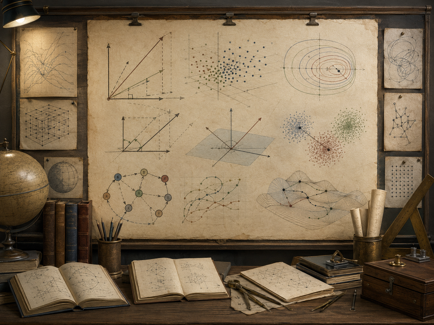
State space is not just a collection of possible system states. It becomes geometrically meaningful only when the model defines how states are compared. Inner products define alignment and angle. Norms define length and magnitude. Distances define separation between states. These choices determine how a model measures similarity, error, deviation, residuals, change, risk, and approximation quality.
For systems modeling, geometry is never neutral. A distance measure can privilege one variable over another. A norm can make small deviations look large or large deviations look small. A scaling choice can change which states appear close. A weighted inner product can reflect energy, uncertainty, importance, covariance, cost, or risk. The geometry chosen by the model shapes the conclusions the model can responsibly support.
Why State-Space Geometry Matters
State-space geometry matters because models compare states. A system state may represent temperature readings, economic sector outputs, infrastructure conditions, ecological populations, policy indicators, machine-learning features, or simulation variables. To compare two states, the model must decide what counts as difference, similarity, magnitude, and change.
Those decisions are mathematical, but they are also substantive. If one variable is measured in dollars and another in tons, ordinary Euclidean distance may be meaningless without scaling. If one measurement is highly uncertain and another is reliable, a weighted geometry may be more appropriate. If outliers matter differently from average deviations, different norms can produce different conclusions.
| Geometric concept | Linear algebra role | Systems modeling interpretation |
|---|---|---|
| Inner product | Defines alignment and angle. | Measures whether state directions reinforce, oppose, or separate. |
| Norm | Defines vector length or magnitude. | Measures size of a state, deviation, residual, or change. |
| Distance | Defines separation between states. | Measures how different two system states are. |
| Weighting | Changes geometric importance of directions. | Reflects units, uncertainty, risk, energy, cost, or domain priority. |
| Scaling | Changes coordinate magnitude. | Determines whether variables are comparable in distance calculations. |
State-space geometry determines what a model treats as close, far, large, small, aligned, independent, or anomalous.
Vectors Need Geometry
A vector space supports addition and scalar multiplication. But those operations alone do not define length, angle, or distance. To speak about the size of a vector, the angle between vectors, or the distance between states, additional structure is required.
This is why inner products and norms are not decorative. They define the geometry of the model. Two models may use the same state variables but different geometries, leading to different measures of error, similarity, and importance.
| Vector-space operation | What it allows | What it does not define by itself |
|---|---|---|
| Addition | Combine states or changes. | Length, angle, distance, or similarity. |
| Scalar multiplication | Scale a state or direction. | Magnitude meaning without a norm. |
| Linear combination | Build states from basis directions. | Which combination is close to another state. |
| Subspace | Represent allowed or modeled directions. | Closest point without a distance measure. |
| Basis | Give coordinates. | Whether coordinate axes are equally meaningful. |
\text{Vector space}+\text{inner product}\Longrightarrow\text{geometry}
\]
Interpretation: Inner products and norms turn algebraic state spaces into geometric spaces where alignment, length, and distance can be measured.
Choosing the geometry is therefore part of the modeling design.
Inner Products
An inner product is a rule that takes two vectors and returns a scalar. It generalizes the dot product and defines alignment, angle, orthogonality, and length. In real vector spaces, an inner product is usually written as \(\langle \mathbf{x},\mathbf{y}\rangle\).
\langle \mathbf{x},\mathbf{y}\rangle
\]
Interpretation: An inner product measures how two vectors align under the chosen geometry.
For real vector spaces, an inner product must satisfy several core properties: symmetry, linearity in one argument, and positive definiteness.
| Property | Formal expression | Modeling interpretation |
|---|---|---|
| Symmetry | \(\langle \mathbf{x},\mathbf{y}\rangle=\langle \mathbf{y},\mathbf{x}\rangle\) | Alignment is mutual under the chosen geometry. |
| Linearity | \(\langle a\mathbf{x}+b\mathbf{z},\mathbf{y}\rangle=a\langle\mathbf{x},\mathbf{y}\rangle+b\langle\mathbf{z},\mathbf{y}\rangle\) | Alignment respects linear combination. |
| Positive definiteness | \(\langle \mathbf{x},\mathbf{x}\rangle>0\) for \(\mathbf{x}\neq\mathbf{0}\) | Nonzero states have positive size. |
| Zero self-product | \(\langle \mathbf{x},\mathbf{x}\rangle=0\Rightarrow \mathbf{x}=\mathbf{0}\) | Only the zero state has zero magnitude. |
| Orthogonality | \(\langle \mathbf{x},\mathbf{y}\rangle=0\) | Directions are separated under the chosen geometry. |
The inner product defines what it means for state directions to overlap.
The Dot Product
The standard dot product is the most familiar inner product on real coordinate vectors. For vectors \(\mathbf{x},\mathbf{y}\in\mathbb{R}^n\), it is:
\mathbf{x}\cdot\mathbf{y}
=
x_1y_1+x_2y_2+\cdots+x_ny_n
\]
Interpretation: The dot product adds coordinate-wise products to measure alignment under the standard Euclidean geometry.
The dot product is simple and powerful, but it assumes the coordinate dimensions are already comparable. If variables use different units or scales, the standard dot product may produce misleading geometry.
| Dot-product assumption | Why it matters | Systems modeling caution |
|---|---|---|
| Comparable coordinates | Each coordinate contributes directly to alignment. | Variables with different units may dominate unfairly. |
| Equal weighting | All dimensions are treated equally unless scaled. | Equal mathematical weight may not match domain importance. |
| Euclidean geometry | Distance and angle follow standard coordinate geometry. | Euclidean closeness may not match system meaning. |
| Coordinate representation | Dot products depend on how states are encoded. | Change of basis or scaling can change alignment measures. |
| No covariance adjustment | Correlated variables are not automatically handled. | Redundant directions can distort similarity and distance. |
The dot product is a default geometry, not a universally correct geometry.
Angles and Alignment
Inner products define angles. In Euclidean geometry, the angle \(\theta\) between nonzero vectors \(\mathbf{x}\) and \(\mathbf{y}\) satisfies:
\cos(\theta)=
\frac{\mathbf{x}\cdot\mathbf{y}}{\|\mathbf{x}\|_2\|\mathbf{y}\|_2}
\]
Interpretation: The normalized dot product measures directional alignment independent of vector magnitude.
This quantity is often called cosine similarity in data analysis and machine learning. It compares direction rather than size. Two large vectors and two small vectors can have the same angle if they point in the same direction.
| Cosine value | Geometric meaning | Systems modeling interpretation |
|---|---|---|
| Near \(1\) | Vectors point in similar directions. | States have similar composition or pattern. |
| Near \(0\) | Vectors are nearly orthogonal. | States are separated under the chosen geometry. |
| Near \(-1\) | Vectors point in opposite directions. | States express opposing patterns. |
| Undefined for zero vector | Angle requires nonzero magnitude. | Zero or near-zero states require careful handling. |
| Scale-invariant | Magnitude is removed. | Useful when direction matters more than size. |
Alignment is useful when the shape or pattern of a state matters more than its magnitude.
Weighted Inner Products
A weighted inner product changes the geometry by assigning different importance to different directions. If \(W\) is a symmetric positive definite matrix, a weighted inner product can be written as:
\langle \mathbf{x},\mathbf{y}\rangle_W=\mathbf{x}^TW\mathbf{y}
\]
Interpretation: The matrix \(W\) defines how directions are weighted when measuring alignment.
If \(W\) is diagonal, each coordinate receives a separate weight. If \(W\) has off-diagonal entries, the geometry can also account for relationships among variables.
| Weighting choice | Mathematical effect | Systems modeling interpretation |
|---|---|---|
| Identity matrix | Standard Euclidean geometry. | All coordinates are treated equally after encoding. |
| Diagonal weights | Coordinates receive different importance. | Reflects units, reliability, priority, cost, or risk. |
| Large weight | Deviation in that direction matters more. | Small changes may be treated as significant. |
| Small weight | Deviation in that direction matters less. | Variation may be treated as lower priority or less reliable. |
| Full positive definite matrix | Geometry includes cross-variable coupling. | Correlations or system relationships affect distance and alignment. |
Weighted inner products make geometry explicit, but the weights must be justified.
Norms
A norm measures the magnitude or length of a vector. Norms are often derived from inner products, but not every norm comes from an inner product. A norm is usually written as \(\|\mathbf{x}\|\).
\|\mathbf{x}\|=\text{size or magnitude of }\mathbf{x}
\]
Interpretation: A norm assigns a nonnegative magnitude to a vector, residual, state, or change.
A norm must satisfy positivity, homogeneity, and the triangle inequality.
| Norm property | Formal expression | Modeling interpretation |
|---|---|---|
| Nonnegativity | \(\|\mathbf{x}\|\geq0\) | Magnitude cannot be negative. |
| Definiteness | \(\|\mathbf{x}\|=0\Rightarrow\mathbf{x}=\mathbf{0}\) | Only the zero state has zero size. |
| Homogeneity | \(\|a\mathbf{x}\|=|a|\|\mathbf{x}\|\) | Scaling a state scales its magnitude proportionally. |
| Triangle inequality | \(\|\mathbf{x}+\mathbf{y}\|\leq\|\mathbf{x}\|+\|\mathbf{y}\|\) | Combined change is no larger than the sum of component changes. |
| Geometry choice | Different norms define different shapes. | Magnitude depends on the modeling geometry. |
Norms are used to measure residual size, error, state change, perturbation, convergence, distance from equilibrium, and sensitivity.
Common Vector Norms
Different norms emphasize different aspects of a vector. The Euclidean norm measures root-sum-square magnitude. The \(1\)-norm measures total absolute magnitude. The infinity norm measures the largest absolute coordinate. General \(p\)-norms interpolate among these behaviors.
\|\mathbf{x}\|_1=\sum_i |x_i|,
\qquad
\|\mathbf{x}\|_2=\sqrt{\sum_i x_i^2},
\qquad
\|\mathbf{x}\|_\infty=\max_i |x_i|
\]
Interpretation: Different norms measure vector magnitude in different ways, emphasizing total deviation, Euclidean magnitude, or maximum coordinate deviation.
| Norm | Formula | What it emphasizes | Modeling use |
|---|---|---|---|
| \(1\)-norm | \(\sum_i |x_i|\) | Total absolute deviation. | Aggregate burden, total error, sparse modeling contexts. |
| \(2\)-norm | \(\sqrt{\sum_i x_i^2}\) | Euclidean magnitude. | Least squares, geometry, residual magnitude, energy-like measures. |
| \(\infty\)-norm | \(\max_i |x_i|\) | Worst coordinate deviation. | Maximum error, safety threshold, robust constraint review. |
| Weighted norm | \(\sqrt{\mathbf{x}^TW\mathbf{x}}\) | Weighted magnitude. | Risk, uncertainty, reliability, energy, cost, or policy priority. |
| General \(p\)-norm | \((\sum_i |x_i|^p)^{1/p}\) | Adjustable deviation emphasis. | Model-dependent error and regularization design. |
The norm chosen for a model determines which deviations matter most.
Distance Between States
Distance between two state vectors is usually measured by applying a norm to their difference. If \(\mathbf{x}\) and \(\mathbf{y}\) are two system states, then:
d(\mathbf{x},\mathbf{y})=\|\mathbf{x}-\mathbf{y}\|
\]
Interpretation: Distance measures the magnitude of the change or difference between two states.
This formula is simple, but its meaning depends entirely on the norm. Different norms can produce different judgments about which states are close, which are far, and which changes are important.
| Distance question | Possible norm | Interpretation |
|---|---|---|
| How large is the overall deviation? | \(2\)-norm | Euclidean magnitude of state difference. |
| How large is the total absolute deviation? | \(1\)-norm | Aggregate difference across all coordinates. |
| What is the worst coordinate deviation? | \(\infty\)-norm | Largest single coordinate difference. |
| How costly is this deviation? | Weighted norm | Distance reflects cost, risk, energy, or importance. |
| How unusual is this deviation statistically? | Covariance-aware norm | Distance accounts for variance and correlation. |
Distance is not just subtraction. It is subtraction plus a chosen geometry.
Residuals and Error Magnitude
Residuals are difference vectors. They measure the gap between what was observed and what a model produced. If \(\mathbf{b}\) is the observed target and \(\widehat{\mathbf{b}}\) is the fitted or modeled value, then:
\mathbf{r}=\mathbf{b}-\widehat{\mathbf{b}}
\]
Interpretation: A residual vector records the direction and magnitude of what the model did not capture.
To summarize residual size, a norm is applied:
\|\mathbf{r}\|
\]
Interpretation: A residual norm measures the size of model mismatch under the chosen geometry.
Different residual norms tell different stories. The \(2\)-norm emphasizes squared deviations. The \(1\)-norm is less dominated by large outliers. The infinity norm focuses on worst-case deviation. A weighted norm can account for uncertainty, reliability, priority, or consequence.
| Residual norm | Modeling meaning | Caution |
|---|---|---|
| \(\|\mathbf{r}\|_2\) | Euclidean mismatch magnitude. | Large errors receive strong influence through squaring. |
| \(\|\mathbf{r}\|_1\) | Total absolute mismatch. | May be less sensitive to isolated large errors. |
| \(\|\mathbf{r}\|_\infty\) | Worst coordinate mismatch. | Useful for safety thresholds, but ignores aggregate pattern. |
| \(\|\mathbf{r}\|_W\) | Weighted mismatch. | Weights must be justified and documented. |
| Normalized residual | Mismatch relative to scale. | Normalization changes interpretive units. |
A residual norm is not an objective truth about model quality. It is a measurement under a chosen geometry.
Scaling, Units, and Normalization
Scaling affects geometry. If one coordinate is measured in millions and another in fractions, ordinary distance will often be dominated by the large-scale coordinate. This may reflect reality, or it may be a unit artifact.
Normalization and standardization change coordinates so that variables become more comparable. But they also change interpretation. A standardized variable no longer represents the original unit directly; it represents deviation relative to a reference distribution.
\tilde{x}_i=\frac{x_i-\mu_i}{\sigma_i}
\]
Interpretation: Standardization expresses a coordinate as deviation from a reference mean in units of reference standard deviation.
| Scaling choice | Purpose | Interpretive caution |
|---|---|---|
| Raw units | Preserve original measurement meaning. | Distance may be dominated by high-magnitude units. |
| Unit conversion | Use consistent measurement units. | Coefficients and distances change numerically. |
| Normalization | Place variables on comparable ranges. | Original units become less visible. |
| Standardization | Compare deviations relative to distribution. | Depends on reference sample and may shift over time. |
| Nondimensionalization | Remove physical units using characteristic scales. | Requires justified characteristic quantities. |
Scaling choices should be treated as modeling assumptions, not preprocessing details.
State-Space Distance and Model Meaning
In state-space modeling, a state vector represents the condition of a system at a moment, scenario, or simulation step. Distance between states can mean physical change, economic difference, ecological shift, infrastructure degradation, policy movement, or feature-space separation.
But distance only has meaning relative to the state representation. If coordinates are poorly chosen, scaled inconsistently, or mixed across incompatible units, state-space distance may be misleading.
| State-space question | Distance interpretation | Required review |
|---|---|---|
| How far did the system move? | Magnitude of state change. | Check units, scaling, and norm choice. |
| How similar are two scenarios? | Distance between scenario vectors. | Check whether all coordinates are comparable. |
| How large is the model error? | Residual norm. | Check weighting and uncertainty. |
| How unusual is this state? | Distance from reference state or distribution. | Check baseline and covariance structure. |
| How close is the system to a threshold? | Distance to boundary or constraint. | Check threshold geometry and decision context. |
Distance in state space is useful only when the state-space representation is meaningful.
Energy, Risk, and Weighted Geometry
In many systems, ordinary Euclidean geometry is not the most meaningful geometry. A weighted norm may better represent energy, cost, uncertainty, reliability, priority, exposure, or risk.
\|\mathbf{x}\|_W=\sqrt{\mathbf{x}^TW\mathbf{x}}
\]
Interpretation: A weighted norm measures vector magnitude under a geometry defined by the positive definite matrix \(W\).
If a deviation in one coordinate is more costly or more dangerous than a deviation in another, a weighted norm can express that difference. But weights embed judgment. They should be documented and reviewed.
| Weighted geometry use | Possible interpretation | Governance question |
|---|---|---|
| Energy norm | Magnitude reflects physical energy or system work. | Does the weight matrix match the physics? |
| Risk norm | Magnitude reflects consequence-weighted deviation. | Who defines the consequences and weights? |
| Uncertainty weighting | Less reliable measurements receive lower weight. | Are uncertainty estimates defensible? |
| Cost weighting | Distance reflects economic or operational cost. | Do costs include externalities and distributional effects? |
| Priority weighting | Some dimensions matter more for the decision. | Are priorities transparent and accountable? |
Weighted geometry can make a model more realistic, but it also makes value choices explicit.
Covariance-Aware Distance
When variables have different variances or are correlated, covariance-aware distance can be more meaningful than ordinary Euclidean distance. One common form is the Mahalanobis distance. If \(\Sigma\) is a covariance matrix, then the squared Mahalanobis distance from \(\boldsymbol{\mu}\) is:
d_M^2(\mathbf{x},\boldsymbol{\mu})
=
(\mathbf{x}-\boldsymbol{\mu})^T\Sigma^{-1}(\mathbf{x}-\boldsymbol{\mu})
\]
Interpretation: Mahalanobis distance measures how unusual a state is relative to covariance structure, not just raw coordinate difference.
This distance accounts for scale and correlation. A deviation along a high-variance direction may be less unusual than the same raw deviation along a low-variance direction. Correlated variables are not treated as fully independent dimensions.
| Distance type | What it uses | When it helps | Caution |
|---|---|---|---|
| Euclidean distance | Raw coordinate differences. | Comparable, independent, similarly scaled variables. | Can mislead under different units or correlations. |
| Standardized distance | Scaled coordinate differences. | Variables with different magnitudes. | Ignores cross-variable covariance unless extended. |
| Mahalanobis distance | Covariance matrix inverse. | Correlated variables and anomaly detection. | Requires reliable covariance estimation. |
| Weighted distance | User-defined weight matrix. | Risk, cost, energy, or priority modeling. | Weights embed assumptions and judgments. |
| Domain-specific distance | Problem-defined metric. | Specialized systems with nonstandard geometry. | Requires validation and explanation. |
Covariance-aware distance can improve interpretation when the geometry of variation matters.
Norms and Numerical Conditioning
Norms are central to numerical analysis. They measure vector size, matrix size, perturbation size, residual size, approximation error, and condition numbers. Without norms, numerical stability cannot be quantified.
A matrix norm measures the size of a matrix as an operator. It helps describe how much a matrix can amplify input vectors.
\|A\|=\max_{\mathbf{x}\neq0}\frac{\|A\mathbf{x}\|}{\|\mathbf{x}\|}
\]
Interpretation: An induced matrix norm measures the largest amplification that a matrix can apply to a nonzero input vector.
The condition number of a matrix measures sensitivity to perturbation:
\kappa(A)=\|A\|\,\|A^{-1}\|
\]
Interpretation: A large condition number means that small input or data changes can produce large solution changes.
| Numerical quantity | Norm-based role | Systems modeling interpretation |
|---|---|---|
| Residual norm | Measures mismatch size. | How far model output is from target. |
| Error norm | Measures deviation from known or reference solution. | How large the approximation error is. |
| Matrix norm | Measures operator size. | How strongly a system transformation can amplify state vectors. |
| Condition number | Measures sensitivity. | How fragile a solution or transformation may be. |
| Convergence tolerance | Uses norm threshold. | When an iterative method is considered accurate enough. |
Numerical claims depend on norm choices. A workflow should document which norms were used and why.
Mathematical Deepening
This section adds a more formal layer. Inner products, norms, and distances connect vector spaces, metric spaces, Hilbert spaces, orthogonality, projections, dual norms, induced matrix norms, positive definite matrices, energy norms, covariance geometry, optimization, regularization, stability, convergence, and approximation theory.
Inner Product Structure
Alignment
An inner product measures whether two vectors point together, oppose each other, or separate under the chosen geometry.
Orthogonality
Vectors are orthogonal when their inner product is zero.
Angle
Angles can be defined using inner products and derived norms.
Weighted Geometry
A positive definite matrix can define a geometry that weights directions differently.
Norm Structure
Magnitude
A norm assigns size to states, changes, residuals, and errors.
Norm Equivalence
In finite-dimensional spaces, many norms are equivalent mathematically, but not always interpretively.
Weighted Norms
Weighted norms can encode energy, risk, cost, uncertainty, or importance.
Matrix Norms
Matrix norms measure transformation size and amplification behavior.
Distance Structure
State Difference
Distance usually applies a norm to the difference between two state vectors.
Metric Choice
Different metrics can produce different judgments about closeness and separation.
Covariance Geometry
Covariance-aware distance accounts for scale, variance, and correlation structure.
Threshold Geometry
Distance to a boundary or constraint depends on the chosen norm.
Computational Diagnostics
Residual Norm
Report the norm used to measure model mismatch.
Relative Error
Compare error to reference magnitude when absolute scale is not enough.
Condition Number
Use norm-based condition numbers to assess sensitivity.
Scaling Audit
Check whether units and coordinate magnitudes distort geometry.
Governance Questions
What Counts as Close?
Define the distance measure before interpreting similarity or deviation.
What Counts as Large?
Define the norm before interpreting magnitude or error.
What Is Weighted?
Document whether weights represent units, uncertainty, cost, risk, or priority.
What Is Hidden by Scaling?
Translate normalized or weighted results back into domain terms.
Examples from Systems Modeling
Inner products, norms, and distance appear whenever models compare states, measure errors, assess similarity, or decide whether a change is significant.
Infrastructure Condition States
Distance between asset-condition vectors can measure deterioration, but weights may be needed if some assets are more critical than others.
Economic Sector Profiles
Norms can measure changes in sector output, while cosine similarity can compare economic structure independent of total scale.
Ecological Community States
Distances between population vectors can measure ecological shift, but scaling and species importance affect interpretation.
Climate and Energy Systems
Weighted norms can represent energy, physical units, or grid reliability when comparing scenario states.
Machine Learning Feature Spaces
Similarity and distance in feature space depend on encoding, normalization, embeddings, and metric choice.
Policy Indicator Dashboards
Composite scores depend on distance, weighting, and normalization choices that should be transparent and reviewable.
Across these examples, the geometry used to compare states should be documented as part of the model itself.
Computation and Reproducible Workflows
Computational workflows for inner products, norms, and distance should document the state vectors, coordinate units, scaling method, inner product definition, norm choice, distance metric, residual norm, weighted matrix if used, covariance matrix if used, condition diagnostics, and interpretation warnings.
The companion repository treats state-space geometry as auditable systems modeling. Python, R, Julia, SQL, Haskell, C, C++, Fortran, Rust, Go, notebooks, schemas, generated outputs, Canvas artifacts, advanced reports, and calculators each support a different layer of reproducible geometry analysis.
For this article, the computational examples focus on standard and weighted inner products, vector norms, distance between states, residual norms, scaling warnings, and model-governance records.
Python Workflow: State-Space Geometry Audit
The Python workflow below computes dot products, weighted inner products, common norms, distances, residual magnitudes, cosine similarity, and interpretation warnings.
from __future__ import annotations

from dataclasses import asdict, dataclass
from pathlib import Path
import csv
import json
import math


Vector = list[float]
Matrix = list[list[float]]


@dataclass(frozen=True)
class StateSpaceGeometryAudit:
    system_name: str
    state_a: str
    state_b: str
    difference_vector: str
    dot_product: float
    cosine_similarity: float
    weighted_inner_product: float
    norm_1: float
    norm_2: float
    norm_inf: float
    euclidean_distance: float
    weighted_distance: float
    interpretation_warning: str


def dot(a: Vector, b: Vector) -> float:
    return sum(x * y for x, y in zip(a, b))


def matvec(A: Matrix, x: Vector) -> Vector:
    return [dot(row, x) for row in A]


def weighted_inner_product(x: Vector, y: Vector, W: Matrix) -> float:
    return dot(x, matvec(W, y))


def subtract(a: Vector, b: Vector) -> Vector:
    return [x - y for x, y in zip(a, b)]


def norm1(x: Vector) -> float:
    return sum(abs(v) for v in x)


def norm2(x: Vector) -> float:
    return math.sqrt(sum(v * v for v in x))


def norminf(x: Vector) -> float:
    return max(abs(v) for v in x)


def cosine_similarity(a: Vector, b: Vector) -> float:
    denom = norm2(a) * norm2(b)
    if denom <= 1e-12:
        raise ValueError("cosine similarity undefined for near-zero vector")
    return dot(a, b) / denom


def vector_to_string(x: Vector) -> str:
    return ",".join(f"{v:.6f}" for v in x)


def build_audit() -> StateSpaceGeometryAudit:
    state_a = [12.0, 4.0, 0.8]
    state_b = [10.0, 5.5, 1.1]
    difference = subtract(state_a, state_b)

    # Diagonal weights: third coordinate matters more because it represents
    # a normalized risk or reliability measure in this synthetic example.
    W = [
        [1.0, 0.0, 0.0],
        [0.0, 0.5, 0.0],
        [0.0, 0.0, 8.0],
    ]

    weighted_diff_magnitude = math.sqrt(weighted_inner_product(difference, difference, W))

    return StateSpaceGeometryAudit(
        system_name="three_indicator_state_space_geometry_audit",
        state_a=vector_to_string(state_a),
        state_b=vector_to_string(state_b),
        difference_vector=vector_to_string(difference),
        dot_product=round(dot(state_a, state_b), 12),
        cosine_similarity=round(cosine_similarity(state_a, state_b), 12),
        weighted_inner_product=round(weighted_inner_product(state_a, state_b, W), 12),
        norm_1=round(norm1(difference), 12),
        norm_2=round(norm2(difference), 12),
        norm_inf=round(norminf(difference), 12),
        euclidean_distance=round(norm2(difference), 12),
        weighted_distance=round(weighted_diff_magnitude, 12),
        interpretation_warning=(
            "State-space distance depends on units, scaling, norm choice, and weights. "
            "Weighted distances may reflect risk, uncertainty, cost, or priority, but those weights "
            "must be documented and translated back into domain terms."
        ),
    )


def write_outputs(output_dir: Path) -> None:
    (output_dir / "tables").mkdir(parents=True, exist_ok=True)
    (output_dir / "json").mkdir(parents=True, exist_ok=True)

    audit = build_audit()
    row = asdict(audit)

    with (output_dir / "tables" / "state_space_geometry_audit.csv").open(
        "w", newline="", encoding="utf-8"
    ) as handle:
        writer = csv.DictWriter(handle, fieldnames=list(row.keys()))
        writer.writeheader()
        writer.writerow(row)

    (output_dir / "json" / "state_space_geometry_audit.json").write_text(
        json.dumps(row, indent=2, sort_keys=True),
        encoding="utf-8",
    )


if __name__ == "__main__":
    write_outputs(Path("outputs"))
    print("State-space geometry audit complete.")
This workflow treats geometry as a modeling assumption. It reports multiple norms and distances so that the modeler can see how conclusions depend on measurement choice.
R Workflow: Inner Product and Norm Diagnostics
R can support geometry diagnostics by computing dot products, cosine similarity, common norms, weighted distances, and audit-ready records.
state_a <- c(12.0, 4.0, 0.8)
state_b <- c(10.0, 5.5, 1.1)

difference <- state_a - state_b

dot_product <- sum(state_a * state_b)

norm1 <- function(x) sum(abs(x))
norm2 <- function(x) sqrt(sum(x^2))
norminf <- function(x) max(abs(x))

cosine_similarity <- dot_product / (norm2(state_a) * norm2(state_b))

W <- matrix(
  c(
    1.0, 0.0, 0.0,
    0.0, 0.5, 0.0,
    0.0, 0.0, 8.0
  ),
  nrow = 3,
  byrow = TRUE
)

weighted_inner_product <- as.numeric(t(state_a) %*% W %*% state_b)
weighted_distance <- sqrt(as.numeric(t(difference) %*% W %*% difference))

audit_record <- data.frame(
  system_name = "three_indicator_state_space_geometry_audit",
  state_a = paste(round(state_a, 6), collapse = ","),
  state_b = paste(round(state_b, 6), collapse = ","),
  difference_vector = paste(round(difference, 6), collapse = ","),
  dot_product = dot_product,
  cosine_similarity = cosine_similarity,
  weighted_inner_product = weighted_inner_product,
  norm_1 = norm1(difference),
  norm_2 = norm2(difference),
  norm_inf = norminf(difference),
  euclidean_distance = norm2(difference),
  weighted_distance = weighted_distance,
  interpretation_warning = paste(
    "State-space distance depends on units, scaling, norm choice, and weights.",
    "Weighted distances require documented domain justification."
  )
)

dir.create("outputs/tables", recursive = TRUE, showWarnings = FALSE)

write.csv(
  audit_record,
  "outputs/tables/r_state_space_geometry_audit.csv",
  row.names = FALSE
)

print(audit_record)
This R workflow is useful when comparing scenarios, residuals, indicator states, feature vectors, or system trajectories under different distance assumptions.
Haskell Workflow: Typed Geometry Records
Haskell can represent state-space geometry diagnostics as a typed record with fields for dot products, similarity, norms, distances, and interpretation warnings.
module Main where

data StateSpaceGeometryAudit = StateSpaceGeometryAudit
  { systemName :: String
  , stateA :: String
  , stateB :: String
  , differenceVector :: String
  , dotProduct :: Double
  , cosineSimilarity :: Double
  , weightedInnerProduct :: Double
  , normOne :: Double
  , normTwo :: Double
  , normInfinity :: Double
  , euclideanDistance :: Double
  , weightedDistance :: Double
  , interpretationWarning :: String
  } deriving (Show)

buildAudit :: StateSpaceGeometryAudit
buildAudit =
  StateSpaceGeometryAudit
    "three_indicator_state_space_geometry_audit"
    "12.000000,4.000000,0.800000"
    "10.000000,5.500000,1.100000"
    "2.000000,-1.500000,-0.300000"
    142.88
    0.988725
    133.04
    3.8
    2.517936
    2.0
    2.517936
    2.33538
    "Distance depends on units, scaling, norm choice, and weights; weighted geometry requires domain justification."

main :: IO ()
main =
  print buildAudit
The typed workflow keeps geometry choices attached to interpretation, instead of reducing state-space comparison to anonymous arithmetic.
SQL Workflow: Distance Assumption Registry
SQL can document inner-product, norm, and distance assumptions when state-space geometry supports dashboards, model audits, residual reviews, simulation reports, or institutional decision workflows.
CREATE TABLE state_space_geometry_assumption_registry (
    assumption_key TEXT PRIMARY KEY,
    assumption_name TEXT NOT NULL,
    mathematical_role TEXT NOT NULL,
    systems_modeling_role TEXT NOT NULL,
    review_warning TEXT NOT NULL
);

INSERT INTO state_space_geometry_assumption_registry VALUES
(
  'inner_product',
  'Inner product',
  'Defines alignment, angle, orthogonality, and derived length.',
  'Determines how state directions are compared.',
  'Changing weights, units, or scaling can change geometric conclusions.'
);

INSERT INTO state_space_geometry_assumption_registry VALUES
(
  'norm',
  'Norm',
  'Measures vector magnitude.',
  'Measures state size, residual magnitude, error, or change.',
  'Different norms emphasize different kinds of deviation.'
);

INSERT INTO state_space_geometry_assumption_registry VALUES
(
  'distance',
  'Distance',
  'Applies a norm to the difference between states.',
  'Measures separation between scenarios, observations, or simulations.',
  'Distance is meaningful only when state coordinates are comparable.'
);

INSERT INTO state_space_geometry_assumption_registry VALUES
(
  'weighted_geometry',
  'Weighted geometry',
  'Uses a positive definite matrix to weight directions.',
  'Represents risk, cost, energy, uncertainty, priority, or reliability.',
  'Weights must be justified and documented.'
);

INSERT INTO state_space_geometry_assumption_registry VALUES
(
  'normalization',
  'Normalization',
  'Transforms coordinates to comparable scales.',
  'Reduces unit dominance in distance calculations.',
  'Normalized outputs must be translated back into domain terms.'
);

INSERT INTO state_space_geometry_assumption_registry VALUES
(
  'covariance_distance',
  'Covariance-aware distance',
  'Uses covariance structure to measure unusual deviation.',
  'Accounts for variance and correlation among state variables.',
  'Requires reliable covariance estimation and review.'
);

SELECT
    assumption_name,
    mathematical_role,
    systems_modeling_role,
    review_warning
FROM state_space_geometry_assumption_registry
ORDER BY assumption_key;
This registry keeps state-space geometry tied to inner products, norms, distance, scaling, weighting, covariance, and responsible interpretation.
GitHub Repository
The companion repository for this article is designed as a reproducible mathematical-modeling workspace. It supports inner-product audits, norm comparisons, state-space distance reports, weighted geometry diagnostics, residual norm records, SQL governance tables, generated outputs, advanced mathematical audit reports, and reusable calculator scripts.
Complete Code Repository
Companion article folder with Python, R, Julia, SQL, Haskell, C, C++, Fortran, Rust, Go, notebooks, documentation, synthetic teaching data, generated outputs, schemas, Canvas-ready workflow artifacts, and reusable calculator scripts for inner products, norms, distance in state space, weighted geometry, cosine similarity, residual norms, state comparison, covariance-aware distance, scaling diagnostics, model governance, and responsible mathematical modeling.
Interpretive Limits and Responsible Use
Inner products, norms, and distances are powerful because they make state-space comparison precise. They are limited because precision does not guarantee meaning. A distance can be mathematically valid while being substantively inappropriate. A norm can be easy to compute while emphasizing the wrong kind of error. A weighted geometry can represent real priorities, but it can also hide contested assumptions inside a matrix.
Euclidean distance is especially easy to misuse. It assumes coordinates are comparable after encoding. In real systems, variables may differ in units, uncertainty, scale, reliability, cost, risk, and institutional meaning. Normalization may solve one problem while creating another: transformed coordinates are easier to compare but harder to interpret directly.
Responsible use requires documenting the inner product, norm, metric, scaling method, units, weights, covariance assumptions, residual interpretation, thresholds, tolerances, and whether distance is being used for explanation, approximation, anomaly detection, clustering, forecasting, simulation, optimization, or decision support.
Related Articles
- What Is Linear Algebra for Systems Modeling?
- Scalars, Vectors, and System States
- Vector Spaces and System Representation
- Span, Linear Independence, and Basis
- Dimension and the Structure of Solution Spaces
- Matrices and the Organization of Multivariable Systems
- Matrix Arithmetic and the Logic of Combination
- Systems of Linear Equations
- Gaussian Elimination and Row Reduction
- Pivot Structure and Solvability
- Rank, Nullity, and Structural Dependence
- Determinants and Invertibility
- Inverse Matrices and Structural Recovery
- Overdetermined Systems and Least Squares Thinking
- Linear Transformations and Model Behavior
- Matrix Multiplication and Interaction Effects
- Change of Basis and Alternative Representations
- Projections, Reflections, and Geometric Interpretation
- Orthogonality and Structured Simplification
- Linear Algebra for Systems Modeling
- Mathematical Modeling
- Systems Modeling
- Scientific Computing for Systems Modeling
Further Reading
- Axler, S. (2024) Linear Algebra Done Right. 4th edn. Cham: Springer. Available at: https://linear.axler.net/.
- Boyd, S. and Vandenberghe, L. (2018) Introduction to Applied Linear Algebra: Vectors, Matrices, and Least Squares. Cambridge: Cambridge University Press. Available at: https://vmls-book.stanford.edu/.
- Boyd, S. and Vandenberghe, L. (2018) Introduction to Applied Linear Algebra: Vectors, Matrices, and Least Squares. PDF edition. Stanford University and UCLA. Available at: https://web.stanford.edu/~boyd/vmls/vmls.pdf.
- Georgia Institute of Technology (n.d.) Interactive Linear Algebra. Georgia Institute of Technology. Available at: https://textbooks.math.gatech.edu/ila/.
- Golub, G.H. and Van Loan, C.F. (2013) Matrix Computations. 4th edn. Baltimore, MD: Johns Hopkins University Press. Available at: https://www.press.jhu.edu/books/title/10678/matrix-computations.
- Hefferon, J. (n.d.) Linear Algebra. Saint Michael’s College. Available at: https://joshua.smcvt.edu/linearalgebra/.
- Higham, N.J. (2002) Accuracy and Stability of Numerical Algorithms. 2nd edn. Philadelphia, PA: Society for Industrial and Applied Mathematics. Available at: https://epubs.siam.org/doi/book/10.1137/1.9780898718027.
- Horn, R.A. and Johnson, C.R. (2013) Matrix Analysis. 2nd edn. Cambridge: Cambridge University Press. Available at: https://www.cambridge.org/highereducation/books/matrix-analysis/FDA3627DC2B9F5C3DF2FD8C3CC136B48.
- Julia Documentation (n.d.) Linear Algebra — Julia Standard Library. Julia Documentation. Available at: https://docs.julialang.org/en/v1/stdlib/LinearAlgebra/.
- Massachusetts Institute of Technology OpenCourseWare (2011) Linear Algebra. Cambridge, MA: MIT OpenCourseWare. Available at: https://ocw.mit.edu/courses/18-06sc-linear-algebra-fall-2011/.
- Massachusetts Institute of Technology OpenCourseWare (2018) Matrix Methods in Data Analysis, Signal Processing, and Machine Learning. Cambridge, MA: MIT OpenCourseWare. Available at: https://ocw.mit.edu/courses/18-065-matrix-methods-in-data-analysis-signal-processing-and-machine-learning-spring-2018/.
- Meyer, C.D. (2023) Matrix Analysis and Applied Linear Algebra. 2nd edn. Philadelphia, PA: Society for Industrial and Applied Mathematics. Available at: https://epubs.siam.org/doi/book/10.1137/1.9781611977448.
- MIT Mathematics (2023) Introduction to Linear Algebra, Sixth Edition. Cambridge, MA: Massachusetts Institute of Technology. Available at: https://math.mit.edu/~gs/linearalgebra/ila6/indexila6.html.
- Netlib (n.d.) BLAS — Basic Linear Algebra Subprograms. Netlib Repository. Available at: https://www.netlib.org/blas/.
- Netlib (n.d.) LAPACK — Linear Algebra PACKage. Netlib Repository. Available at: https://www.netlib.org/lapack/.
- Netlib and SIAM (1999) LAPACK Users’ Guide. 3rd edn. Philadelphia, PA: Society for Industrial and Applied Mathematics. Available at: https://www.netlib.org/lapack/lug/.
- NumPy Developers (n.d.) Linear Algebra: numpy.linalg. NumPy Documentation. Available at: https://numpy.org/doc/stable/reference/routines.linalg.html.
- SciPy Developers (n.d.) Linear Algebra: scipy.linalg. SciPy Documentation. Available at: https://docs.scipy.org/doc/scipy/reference/linalg.html.
- Strang, G. (2016) Introduction to Linear Algebra. Wellesley, MA: Wellesley-Cambridge Press. Available at: https://math.mit.edu/~gs/linearalgebra/.
- Treil, S. (2017) Linear Algebra Done Wrong. Providence, RI: Brown University. Available at: https://www.math.brown.edu/streil/papers/LADW/LADW.html.
- Trefethen, L.N. and Bau, D. (1997) Numerical Linear Algebra. Philadelphia, PA: Society for Industrial and Applied Mathematics. Available at: https://epubs.siam.org/doi/book/10.1137/1.9780898719574.
- van de Geijn, R. and Myers, M. (n.d.) Linear Algebra: Foundations to Frontiers. Austin, TX: The University of Texas at Austin. Available at: https://www.cs.utexas.edu/~flame/laff/laff/LAFF-2.00M.pdf.
References
- Axler, S. (2024) Linear Algebra Done Right. 4th edn. Cham: Springer. Available at: https://linear.axler.net/.
- Boyd, S. and Vandenberghe, L. (2018) Introduction to Applied Linear Algebra: Vectors, Matrices, and Least Squares. Cambridge: Cambridge University Press. Available at: https://vmls-book.stanford.edu/.
- Georgia Institute of Technology (n.d.) Interactive Linear Algebra. Georgia Institute of Technology. Available at: https://textbooks.math.gatech.edu/ila/.
- Golub, G.H. and Van Loan, C.F. (2013) Matrix Computations. 4th edn. Baltimore, MD: Johns Hopkins University Press. Available at: https://www.press.jhu.edu/books/title/10678/matrix-computations.
- Hefferon, J. (n.d.) Linear Algebra. Saint Michael’s College. Available at: https://joshua.smcvt.edu/linearalgebra/.
- Higham, N.J. (2002) Accuracy and Stability of Numerical Algorithms. 2nd edn. Philadelphia, PA: Society for Industrial and Applied Mathematics. Available at: https://epubs.siam.org/doi/book/10.1137/1.9780898718027.
- Horn, R.A. and Johnson, C.R. (2013) Matrix Analysis. 2nd edn. Cambridge: Cambridge University Press. Available at: https://www.cambridge.org/highereducation/books/matrix-analysis/FDA3627DC2B9F5C3DF2FD8C3CC136B48.
- Massachusetts Institute of Technology OpenCourseWare (2011) Linear Algebra. Cambridge, MA: MIT OpenCourseWare. Available at: https://ocw.mit.edu/courses/18-06sc-linear-algebra-fall-2011/.
- Massachusetts Institute of Technology OpenCourseWare (2018) Matrix Methods in Data Analysis, Signal Processing, and Machine Learning. Cambridge, MA: MIT OpenCourseWare. Available at: https://ocw.mit.edu/courses/18-065-matrix-methods-in-data-analysis-signal-processing-and-machine-learning-spring-2018/.
- Meyer, C.D. (2023) Matrix Analysis and Applied Linear Algebra. 2nd edn. Philadelphia, PA: Society for Industrial and Applied Mathematics. Available at: https://epubs.siam.org/doi/book/10.1137/1.9781611977448.
- MIT Mathematics (2023) Introduction to Linear Algebra, Sixth Edition. Cambridge, MA: Massachusetts Institute of Technology. Available at: https://math.mit.edu/~gs/linearalgebra/ila6/indexila6.html.
- Netlib (n.d.) BLAS — Basic Linear Algebra Subprograms. Netlib Repository. Available at: https://www.netlib.org/blas/.
- Netlib (n.d.) LAPACK — Linear Algebra PACKage. Netlib Repository. Available at: https://www.netlib.org/lapack/.
- NumPy Developers (n.d.) Linear Algebra: numpy.linalg. NumPy Documentation. Available at: https://numpy.org/doc/stable/reference/routines.linalg.html.
- R Core Team and Matrix Package Authors (n.d.) Matrix: Sparse and Dense Matrix Classes and Methods. CRAN. Available at: https://cran.r-project.org/package=Matrix.
- SciPy Developers (n.d.) Linear Algebra: scipy.linalg. SciPy Documentation. Available at: https://docs.scipy.org/doc/scipy/reference/linalg.html.
- Strang, G. (2016) Introduction to Linear Algebra. Wellesley, MA: Wellesley-Cambridge Press. Available at: https://math.mit.edu/~gs/linearalgebra/.
- Treil, S. (2017) Linear Algebra Done Wrong. Providence, RI: Brown University. Available at: https://www.math.brown.edu/streil/papers/LADW/LADW.html.
- Trefethen, L.N. and Bau, D. (1997) Numerical Linear Algebra. Philadelphia, PA: Society for Industrial and Applied Mathematics. Available at: https://epubs.siam.org/doi/book/10.1137/1.9780898719574.
- van de Geijn, R. and Myers, M. (n.d.) Linear Algebra: Foundations to Frontiers. Austin, TX: The University of Texas at Austin. Available at: https://www.cs.utexas.edu/~flame/laff/laff/LAFF-2.00M.pdf.