
Last Updated June 28, 2026
Change of basis and alternative representations explain how the same system can look different when described in different coordinates. A vector is not only a list of numbers. Those numbers mean something only after a basis has been chosen. A matrix is not only a transformation. Its entries depend on the coordinate system used to represent inputs and outputs.
This article is a deep dive into basis changes, coordinate representations, similarity transformations, transformed matrices, invariant structure, numerical conditioning, scaling choices, and responsible systems interpretation. It connects basis vectors, coordinate maps, change-of-basis matrices, alternative representations, diagonalization previews, principal directions, rotated coordinate systems, orthonormal bases, nonorthogonal bases, units, dimensional scaling, interpretability, and model governance.
The central modeling question is not only “What are the coordinates?” It is “What representation makes the system structure visible without distorting the meaning of the model?”
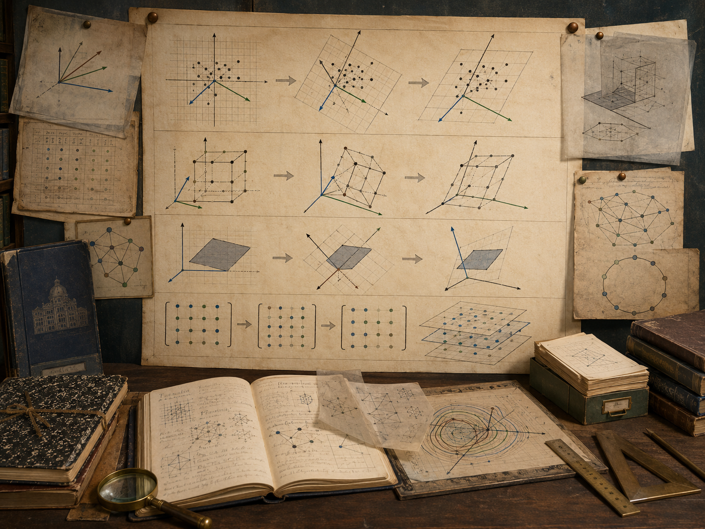
Change of basis is one of the most important ideas in linear algebra because it separates the system from the language used to describe it. A vector may represent the same state whether it is described in standard coordinates, principal directions, normalized variables, eigenvector coordinates, sectoral categories, feature embeddings, or a physically meaningful coordinate frame. The numbers change. The underlying object does not.
For systems modeling, this distinction is crucial. Representation choices affect interpretability, numerical stability, visual clarity, compression, approximation, and decision use. A poor basis can make structure look complicated. A better basis can reveal conservation, independence, dominant modes, weak directions, dependencies, symmetries, or hidden coupling.
Why Change of Basis Matters
Change of basis matters because coordinates are not the system itself. Coordinates are a language for describing the system. The same vector, transformation, or state space can be represented in many different coordinate systems. Some representations make structure visible. Others hide it.
In systems modeling, basis choice can determine whether a model appears coupled or decoupled, stable or unstable, sparse or dense, interpretable or opaque, well-scaled or numerically fragile. A basis can align with physical components, statistical variation, network modes, eigenvectors, policy categories, economic sectors, spatial directions, or computational convenience.
\mathbf{x}=P[\mathbf{x}]_{\mathcal{B}}
\]
Interpretation: A coordinate vector \([\mathbf{x}]_{\mathcal{B}}\) describes the same object \(\mathbf{x}\) using the basis \(\mathcal{B}\), with \(P\) translating basis coordinates into standard coordinates.
The point of changing basis is not cosmetic. It changes the representation so that the structure of interest becomes easier to analyze, compute, compare, or interpret.
| Representation issue | Why it matters | Systems modeling interpretation |
|---|---|---|
| Different coordinates | The same vector has different numerical descriptions. | State meaning depends on the chosen basis. |
| Different matrix entries | The same transformation can look different. | Model behavior may appear simpler or more complex. |
| Alternative basis | New directions organize the state space. | Dominant modes, independent patterns, or structural components may emerge. |
| Similarity transformation | Transformation is rewritten in a new coordinate language. | Underlying behavior is preserved while the representation changes. |
| Conditioning | Some bases are numerically fragile. | Representation can affect computational reliability. |
Change of basis is therefore both mathematical and interpretive. It asks how the same structure should be represented for the purpose at hand.
Coordinates Are Representations
A vector is an object in a vector space. A coordinate list is a representation of that object relative to a basis. This distinction is easy to miss because many introductory examples use the standard basis by default. But once alternative bases enter the picture, the distinction becomes essential.
For example, the coordinate vector \((3,2)\) means different things depending on the basis. In the standard basis, it means \(3\mathbf{e}_1+2\mathbf{e}_2\). In another basis, it means \(3\mathbf{b}_1+2\mathbf{b}_2\). The same numbers can represent different vectors, and the same vector can be represented by different numbers.
[\mathbf{x}]_{\mathcal{B}}=
\begin{pmatrix}
c_1\\
c_2\\
\vdots\\
c_n
\end{pmatrix}
\quad\Longleftrightarrow\quad
\mathbf{x}=c_1\mathbf{b}_1+c_2\mathbf{b}_2+\cdots+c_n\mathbf{b}_n
\]
Interpretation: Coordinates describe how much of each basis vector is used to build the vector.
| Object | Coordinate-dependent? | Systems modeling interpretation |
|---|---|---|
| Vector as system state | No | The underlying state is the object being represented. |
| Coordinate list | Yes | The numerical description depends on the chosen basis. |
| Basis | Yes | The representation language used for states. |
| Transformation behavior | No, at the structural level | The system action exists independently of coordinates. |
| Matrix entries | Yes | The representation of the transformation depends on basis choices. |
Good modeling practice separates the system state from the coordinate description of that state.
Basis Vectors and Coordinate Language
A basis is a set of linearly independent vectors that spans a vector space. It gives every vector in the space a unique coordinate representation. If \(\mathcal{B}=\{\mathbf{b}_1,\ldots,\mathbf{b}_n\}\) is a basis for an \(n\)-dimensional vector space, every vector \(\mathbf{x}\) can be written uniquely as a linear combination of the basis vectors.
\mathbf{x}=c_1\mathbf{b}_1+c_2\mathbf{b}_2+\cdots+c_n\mathbf{b}_n
\]
Interpretation: A basis supplies the coordinate language used to describe system states.
The uniqueness of this representation is what makes coordinates useful. Without independence, different coordinate lists could represent the same vector. Without span, some vectors could not be represented at all.
| Basis requirement | Formal meaning | Modeling consequence |
|---|---|---|
| Spanning | Every vector in the space can be represented. | The representation can describe all relevant states. |
| Linear independence | No basis vector is redundant. | Coordinates are unique and not overdetermined. |
| Dimension match | The basis has \(n\) vectors for an \(n\)-dimensional space. | The representation has the correct number of degrees of freedom. |
| Interpretability | Basis directions may have domain meaning. | Coordinates can be tied to physical, economic, ecological, or policy concepts. |
| Numerical stability | Basis vectors should not be nearly dependent. | Coordinates should not be hypersensitive to small perturbations. |
Basis vectors define what the coordinate axes mean. Changing basis changes the language of representation.
The Change-of-Basis Matrix
A change-of-basis matrix stores the new basis vectors as columns. If \(\mathcal{B}=\{\mathbf{b}_1,\mathbf{b}_2,\ldots,\mathbf{b}_n\}\), then the matrix \(P_{\mathcal{B}}\) is:
P_{\mathcal{B}}=
\begin{pmatrix}
| & | & & |\\
\mathbf{b}_1 & \mathbf{b}_2 & \cdots & \mathbf{b}_n\\
| & | & & |
\end{pmatrix}
\]
Interpretation: The columns of \(P_{\mathcal{B}}\) are the basis vectors written in standard coordinates.
This matrix translates coordinates in the \(\mathcal{B}\)-basis into standard coordinates. It is invertible exactly when the proposed basis vectors are linearly independent and span the space.
\det(P_{\mathcal{B}})\neq 0
\quad\Longleftrightarrow\quad
\mathcal{B}\text{ is a basis}
\]
Interpretation: The basis matrix must be invertible for coordinate translation to be unique and reversible.
| Matrix object | Formal role | Systems modeling interpretation |
|---|---|---|
| \(P_{\mathcal{B}}\) | Basis matrix. | Translates alternative coordinates into the standard representation. |
| Columns of \(P_{\mathcal{B}}\) | Basis vectors. | Alternative system directions, modes, components, or coordinate axes. |
| \(P_{\mathcal{B}}^{-1}\) | Inverse coordinate map. | Translates standard coordinates into basis coordinates. |
| \(\det(P_{\mathcal{B}})\) | Invertibility signal for square basis matrix. | Detects whether the proposed coordinate system collapses structure. |
| \(\kappa(P_{\mathcal{B}})\) | Condition number. | Indicates coordinate sensitivity and numerical fragility. |
The change-of-basis matrix is therefore a translation device between coordinate languages.
From Basis Coordinates to Standard Coordinates
If a vector is given in basis coordinates, the basis matrix converts it into standard coordinates. Suppose \([\mathbf{x}]_{\mathcal{B}}\) is the coordinate vector of \(\mathbf{x}\) relative to basis \(\mathcal{B}\). Then:
\mathbf{x}=P_{\mathcal{B}}[\mathbf{x}]_{\mathcal{B}}
\]
Interpretation: Multiply the basis matrix by the coordinate vector to reconstruct the actual vector in standard coordinates.
This operation is a linear combination of the basis columns. The coordinate entries are weights, and the basis vectors are the ingredients.
P_{\mathcal{B}}
\begin{pmatrix}
c_1\\
c_2\\
\vdots\\
c_n
\end{pmatrix}
=
c_1\mathbf{b}_1+c_2\mathbf{b}_2+\cdots+c_n\mathbf{b}_n
\]
Interpretation: Coordinates tell how much of each basis vector contributes to the represented state.
In modeling terms, this might mean reconstructing a physical state from modal coordinates, reconstructing a signal from frequency components, reconstructing a network state from principal patterns, or reconstructing an economic state from transformed sector coordinates.
From Standard Coordinates to Basis Coordinates
To move from standard coordinates into basis coordinates, apply the inverse basis matrix:
[\mathbf{x}]_{\mathcal{B}}=P_{\mathcal{B}}^{-1}\mathbf{x}
\]
Interpretation: The inverse basis matrix finds the coordinates of \(\mathbf{x}\) in the alternative basis.
This is a coordinate recovery problem. Given the vector \(\mathbf{x}\), we solve for the weights \(c_1,\ldots,c_n\) such that:
\mathbf{x}=c_1\mathbf{b}_1+\cdots+c_n\mathbf{b}_n
\]
Interpretation: Coordinate recovery asks how much of each basis direction is needed to build the state.
In serious numerical work, one should often solve \(P_{\mathcal{B}}\mathbf{c}=\mathbf{x}\) using a stable linear solver rather than explicitly computing \(P_{\mathcal{B}}^{-1}\). This is the same computational caution introduced in the article on inverse matrices: formulas are not always the best algorithms.
| Task | Formula | Computational caution |
|---|---|---|
| Basis coordinates to standard coordinates | \(\mathbf{x}=P_{\mathcal{B}}[\mathbf{x}]_{\mathcal{B}}\) | Usually direct matrix-vector multiplication. |
| Standard coordinates to basis coordinates | \([\mathbf{x}]_{\mathcal{B}}=P_{\mathcal{B}}^{-1}\mathbf{x}\) | Prefer solving \(P_{\mathcal{B}}\mathbf{c}=\mathbf{x}\) over explicitly forming the inverse. |
| Basis validation | \(\operatorname{rank}(P_{\mathcal{B}})=n\) | Check rank before using the coordinate system. |
| Fragility review | \(\kappa(P_{\mathcal{B}})\) | Large condition numbers signal unstable coordinates. |
| Interpretability review | Domain-specific | Coordinates must correspond to meaningful system directions. |
Changing basis is a mathematical translation, but the translation must be numerically and substantively defensible.
Transformations Under Change of Basis
A transformation can be represented by different matrices in different bases. Suppose \(A\) is the matrix of a transformation in standard coordinates. To represent the same transformation in basis \(\mathcal{B}\), we translate a basis-coordinate input into standard coordinates, apply \(A\), and then translate the output back into basis coordinates.
[A]_{\mathcal{B}}=P_{\mathcal{B}}^{-1}AP_{\mathcal{B}}
\]
Interpretation: The same transformation can be rewritten in the coordinate language of basis \(\mathcal{B}\).
The right side should be read from right to left:
- \(P_{\mathcal{B}}\) translates basis coordinates into standard coordinates.
- \(A\) applies the transformation in standard coordinates.
- \(P_{\mathcal{B}}^{-1}\) translates the result back into basis coordinates.
[\mathbf{x}]_{\mathcal{B}}
\xrightarrow{P_{\mathcal{B}}}
\mathbf{x}
\xrightarrow{A}
A\mathbf{x}
\xrightarrow{P_{\mathcal{B}}^{-1}}
[A\mathbf{x}]_{\mathcal{B}}
\]
Interpretation: A change of basis wraps the original transformation between coordinate translation and coordinate recovery.
This formula is one of the most important in linear algebra because it shows that matrix entries are representation-dependent. The underlying transformation is the same, but its coordinate description changes.
Similarity Transformations
Matrices \(A\) and \(B\) are similar if there is an invertible matrix \(P\) such that:
B=P^{-1}AP
\]
Interpretation: Similar matrices represent the same linear transformation in different coordinate systems.
Similarity is not equality of entries. It is equality of underlying transformation structure under a coordinate change. Similar matrices have the same determinant, trace, rank, eigenvalues, characteristic polynomial, and invertibility status, even though their entries may look very different.
| Feature | Preserved under similarity? | Modeling interpretation |
|---|---|---|
| Eigenvalues | Yes | Core dynamic rates, growth factors, or modal behavior are preserved. |
| Determinant | Yes | Volume-scaling structure is preserved. |
| Trace | Yes | Sum of diagonal action is preserved. |
| Rank | Yes | Independent transformation structure is preserved. |
| Invertibility | Yes | Reversibility is independent of coordinate representation. |
| Individual entries | No | Coefficient values depend on the chosen basis. |
| Sparsity pattern | Not generally | A simple model in one basis may look dense in another. |
| Interpretability | Not automatically | A mathematically valid basis may be hard to explain in domain terms. |
Similarity transformations help distinguish invariant system behavior from coordinate artifacts.
What Changes and What Stays Invariant
Change of basis forces a central distinction: some features of a model are representation-dependent, while others are invariant. Coordinates, matrix entries, sparsity, and apparent coupling may change. Rank, dimension, determinant, eigenvalues, and structural reachability may be preserved under appropriate transformations.
This distinction matters for interpretation. If a model seems complicated only because the basis is poorly chosen, a different representation may clarify it. If a property is invariant, changing coordinates will not make it disappear.
| Representation-dependent feature | Invariant or structural feature | Systems modeling lesson |
|---|---|---|
| Coordinate values | Underlying vector | The state is not identical to one coordinate description. |
| Matrix entries | Underlying transformation | Coefficient tables depend on representation. |
| Sparsity pattern | Rank and dimension | A sparse or dense appearance may be basis-dependent. |
| Apparent coupling | Invariant subspace structure | Variables may decouple in a better basis. |
| Scaling of coordinates | Physical or structural relation | Units and normalization affect numerical appearance. |
| Diagonal form when available | Eigenvalue structure | Some transformations become simple in modal coordinates. |
Good analysis asks whether a feature belongs to the system or merely to the representation.
Orthonormal and Nonorthogonal Bases
Some bases are easier to work with than others. An orthonormal basis consists of unit vectors that are mutually perpendicular. If \(Q\) is a matrix whose columns form an orthonormal basis, then:
Q^TQ=I,\qquad Q^{-1}=Q^T
\]
Interpretation: For an orthonormal basis, coordinate conversion is especially stable because the inverse is just the transpose.
Orthonormal bases are central to numerical linear algebra because they preserve lengths and angles. They appear in QR decomposition, projections, least squares, principal component analysis, singular value decomposition, Fourier methods, and many scientific-computing workflows.
Nonorthogonal bases can still be valid and useful. They may align with domain-specific directions that are not perpendicular. But nonorthogonal bases can make coordinate recovery more sensitive, especially when the basis vectors are nearly dependent.
| Basis type | Strength | Risk | Modeling interpretation |
|---|---|---|---|
| Standard basis | Simple default coordinates. | May hide natural system structure. | Variables correspond to original components. |
| Orthonormal basis | Stable, length-preserving coordinate behavior. | Basis directions may be abstract. | Useful for numerical stability and decomposition. |
| Eigenbasis | Can diagonalize transformation when available. | May be ill-conditioned or complex-valued. | Reveals modal behavior and repeated transformation structure. |
| Principal-component basis | Aligns with major variation directions. | May obscure original variable meaning. | Useful for compression and latent structure. |
| Domain-specific basis | Interpretable for experts. | May be nonorthogonal or poorly conditioned. | Useful when directions correspond to real mechanisms or categories. |
The best basis depends on the purpose: computation, interpretation, compression, stability, explanation, or decision support.
Scaling, Normalization, and Units
Scaling is a practical form of representation change. A system described in meters may look different from the same system described in kilometers. A dataset with variables measured in dollars, tons, percentages, and counts may produce misleading geometry unless units and scaling are handled carefully.
Normalization, standardization, nondimensionalization, and unit conversion all change coordinate representations. These changes may improve numerical behavior, but they can also alter interpretability.
\tilde{\mathbf{x}}=D^{-1}\mathbf{x}
\]
Interpretation: A diagonal scaling matrix \(D\) changes coordinate magnitudes by rescaling variables.
| Representation change | Purpose | Interpretive caution |
|---|---|---|
| Unit conversion | Express quantities in different units. | Coefficients change even though physical reality does not. |
| Normalization | Put values on comparable scales. | Original units may become less visible. |
| Standardization | Center and scale variables by statistical variation. | Coordinates become relative to dataset distribution. |
| Nondimensionalization | Remove physical units using characteristic scales. | Requires justified reference quantities. |
| Diagonal scaling | Improve numerical conditioning or solver behavior. | Scaled solution must be translated back for interpretation. |
Scaling choices are not neutral. They affect distances, norms, angles, conditioning, coefficient magnitudes, and sometimes model conclusions.
Basis Choice and Model Interpretation
A basis can be chosen for many reasons. A physical basis may align with real components. A statistical basis may align with variation. An eigenbasis may align with dynamic modes. A Fourier basis may align with frequency. A wavelet basis may align with localized structure. A domain-specific basis may align with institutional categories.
No basis is automatically best. The right basis depends on the modeling purpose.
| Modeling purpose | Potential basis choice | Why it may help |
|---|---|---|
| Physical interpretation | Original component basis. | Coordinates correspond to observable quantities. |
| Dynamic behavior | Eigenbasis or modal basis. | Growth, decay, and oscillatory modes may separate. |
| Approximation | Principal-component basis. | Dominant variation can be captured with fewer coordinates. |
| Signal analysis | Fourier or wavelet basis. | Frequency or localized structure becomes visible. |
| Numerical stability | Orthonormal basis. | Coordinate calculations are often more stable. |
| Policy explanation | Domain-specific basis. | Coordinates align with institutions, sectors, regions, or decision categories. |
Representation choice should therefore be documented as part of the modeling method, not treated as a hidden technical detail.
Condition Numbers and Basis Fragility
A basis can be mathematically valid but numerically fragile. If basis vectors are nearly dependent, small changes in the vector may cause large changes in coordinates. This is a conditioning problem.
\kappa(P)=\|P\|\,\|P^{-1}\|
\]
Interpretation: The condition number of the basis matrix measures how sensitive coordinate conversion may be to perturbations.
A large condition number means that the coordinate system is close to collapsing. In practical modeling, this can make basis coordinates unstable, coefficient estimates fragile, and interpretations unreliable.
| Conditioning issue | Mathematical signal | Systems modeling consequence |
|---|---|---|
| Nearly dependent basis vectors | Large \(\kappa(P)\) | Coordinates become hypersensitive. |
| Small determinant magnitude | Near singular basis matrix. | Representation almost collapses dimension. |
| Unstable inverse | Large entries in \(P^{-1}\) | Small measurement errors produce large coordinate errors. |
| Poor scaling | Large magnitude differences among columns. | Numerical algorithms may behave poorly. |
| Misleading precision | Many digits in unstable coordinates. | Output looks exact but may be fragile. |
For engineer-grade modeling, a change of basis should include a conditioning review. A beautiful representation is not useful if it is numerically unstable.
Basis Changes in Systems Modeling
Basis changes appear throughout systems modeling. Sometimes they are explicit, as in modal analysis or principal component analysis. Sometimes they are hidden, as in scaling, normalization, feature engineering, coordinate transformations, index construction, or dimensionality reduction.
In infrastructure modeling, one basis may describe physical assets while another describes service modes or failure modes. In economics, one representation may describe sectors while another describes independent demand patterns or production modes. In ecology, one basis may describe species counts while another describes interaction modes or environmental gradients. In machine learning, feature transformations create new coordinate systems for prediction or representation.
| Modeling domain | Original representation | Alternative representation | Why change basis? |
|---|---|---|---|
| Infrastructure systems | Asset-level variables. | Failure modes, service modes, or network modes. | Reveal vulnerability structure and interdependence. |
| Economic systems | Sector outputs. | Production modes or demand patterns. | Separate dominant intersectoral structures. |
| Ecological systems | Species or resource variables. | Interaction modes or environmental gradients. | Reveal coupled response patterns. |
| Climate and energy systems | Regional measurements. | Spatial modes or principal components. | Compress high-dimensional variation. |
| Machine learning | Raw features. | Embeddings, principal components, or latent factors. | Improve separation, compression, or predictive structure. |
| Policy indicators | Observed metrics. | Composite dimensions or latent factors. | Organize complex indicator systems. |
Alternative representations can clarify a system, but they can also obscure accountability if the transformed coordinates no longer have clear meaning.
Mathematical Deep Dive
This section develops the deeper structure behind change of basis. It connects coordinate isomorphisms, representation matrices, similarity, invariants, diagonalization, orthogonal transformations, conditioning, and model interpretation.
Coordinate Isomorphisms
Abstract Vector
The vector is the underlying object in the vector space, independent of a particular coordinate list.
Coordinate Vector
The coordinate vector \([\mathbf{x}]_{\mathcal{B}}\) is the numerical representation of \(\mathbf{x}\) relative to basis \(\mathcal{B}\).
Basis Matrix
The matrix \(P_{\mathcal{B}}\) maps basis coordinates into standard coordinates.
Inverse Coordinate Map
The inverse \(P_{\mathcal{B}}^{-1}\) maps standard coordinates into coordinates relative to \(\mathcal{B}\).
Similarity and Invariants
Similar Matrices
Matrices \(A\) and \(P^{-1}AP\) represent the same transformation in different coordinate systems.
Eigenvalues
Eigenvalues are preserved under similarity and describe structural transformation behavior.
Trace and Determinant
Trace and determinant remain unchanged under similarity transformations.
Rank
Rank is preserved because coordinate changes do not alter the dimension of reachable output structure.
Diagonalization Preview
Eigenbasis
If a matrix has enough independent eigenvectors, those eigenvectors can form a basis.
Diagonal Representation
In an eigenbasis, a transformation may become diagonal, separating independent modes.
Repeated Transformation
Diagonal form makes powers of a matrix easier to analyze.
Dynamic Interpretation
Diagonalized systems reveal growth, decay, persistence, and modal response.
Orthogonal Transformations
Orthonormal Basis
Basis vectors are mutually perpendicular and have unit length.
Transpose as Inverse
If \(Q\) is orthogonal, then \(Q^{-1}=Q^T\).
Length Preservation
Orthogonal transformations preserve Euclidean length and angle.
Numerical Stability
Orthonormal bases are central to stable algorithms such as QR and SVD.
Representation Governance
Representation Choice
Document why this basis was chosen and what structure it is meant to reveal.
Coordinate Meaning
Explain what transformed coordinates mean in the modeled system.
Conditioning Review
Check whether the basis matrix creates unstable coordinate conversion.
Translation Back
When alternative coordinates are used, explain how results translate back into original system terms.
Examples from Systems Modeling
Change of basis appears whenever the same system is described in a more useful coordinate language.
Infrastructure Failure Modes
An asset-level representation may be transformed into failure-mode coordinates, revealing vulnerability patterns that are not obvious component by component.
Economic Sector Modes
Sector output vectors can be represented in alternative bases that separate dominant production patterns, dependency structures, or demand modes.
Ecological Interaction Gradients
Species or resource variables can be transformed into ecological gradients or interaction modes that clarify system response.
Climate and Energy Data
High-dimensional spatial measurements can be represented in principal directions that capture dominant variation.
Machine Learning Feature Spaces
Raw features can be mapped into embeddings, latent factors, or principal components, changing the coordinate system used for prediction.
Policy Indicator Systems
Multiple indicators can be reorganized into composite dimensions, but transformed coordinates require careful explanation and accountability.
Across these examples, the representation should serve the system question rather than merely make the algebra convenient.
Computation and Reproducible Workflows
Computational workflows for change of basis should document the original coordinates, alternative basis vectors, basis matrix, rank, determinant when applicable, condition estimate, coordinate conversion, reconstruction error, transformed matrix, invariant checks, and interpretive warnings. A coordinate transformation should not be treated as a silent preprocessing step.
The companion repository treats change of basis as auditable systems modeling. Python, R, Julia, SQL, Haskell, C, C++, Fortran, Rust, Go, notebooks, schemas, generated outputs, Canvas artifacts, advanced reports, and calculators each support a different layer of reproducible representation analysis.
For this article, the computational examples focus on basis validation, coordinate conversion, reconstruction, similarity transformation, condition warnings, and model-governance records.
Python Workflow: Change-of-Basis Audit
The Python workflow below validates a basis, converts a vector into basis coordinates, reconstructs the original vector, transforms a matrix into the new basis, and records interpretation warnings.
from __future__ import annotations

from dataclasses import asdict, dataclass
from pathlib import Path
import csv
import json
import math


Matrix = list[list[float]]
Vector = list[float]


@dataclass(frozen=True)
class ChangeOfBasisAudit:
    system_name: str
    basis_shape: str
    basis_rank: int
    basis_determinant: float
    basis_condition_warning: str
    original_vector: str
    basis_coordinates: str
    reconstructed_vector: str
    reconstruction_error: float
    transformed_matrix: str
    invariant_warning: str
    interpretation_warning: str


def matmul(A: Matrix, B: Matrix) -> Matrix:
    return [
        [sum(a * b for a, b in zip(row, col)) for col in zip(*B)]
        for row in A
    ]


def matvec(A: Matrix, x: Vector) -> Vector:
    return [sum(a * b for a, b in zip(row, x)) for row in A]


def det2(A: Matrix) -> float:
    return A[0][0] * A[1][1] - A[0][1] * A[1][0]


def inv2(A: Matrix) -> Matrix:
    determinant = det2(A)
    if abs(determinant) <= 1e-12:
        raise ValueError("basis matrix is singular or numerically unsafe")
    return [
        [A[1][1] / determinant, -A[0][1] / determinant],
        [-A[1][0] / determinant, A[0][0] / determinant],
    ]


def norm2(v: Vector) -> float:
    return math.sqrt(sum(value * value for value in v))


def matrix_to_string(A: Matrix) -> str:
    return ";".join(",".join(f"{value:.6f}" for value in row) for row in A)


def vector_to_string(v: Vector) -> str:
    return ",".join(f"{value:.6f}" for value in v)


def build_audit() -> ChangeOfBasisAudit:
    # Columns are alternative basis vectors.
    P = [
        [2.0, 1.0],
        [1.0, 2.0],
    ]

    x = [5.0, 4.0]

    # Transformation in standard coordinates.
    A = [
        [1.2, 0.3],
        [0.4, 0.9],
    ]

    Pinv = inv2(P)
    coords = matvec(Pinv, x)
    reconstructed = matvec(P, coords)
    reconstruction_error = norm2([a - b for a, b in zip(x, reconstructed)])

    transformed = matmul(matmul(Pinv, A), P)
    determinant = det2(P)
    basis_rank = 2 if abs(determinant) > 1e-12 else 1

    condition_warning = (
        "basis is valid in this teaching example; serious workflows should compute a numerical condition number"
        if abs(determinant) > 1e-8
        else "basis is near singular or unsafe for coordinate interpretation"
    )

    return ChangeOfBasisAudit(
        system_name="two_mode_representation_audit",
        basis_shape="2x2",
        basis_rank=basis_rank,
        basis_determinant=round(determinant, 12),
        basis_condition_warning=condition_warning,
        original_vector=vector_to_string(x),
        basis_coordinates=vector_to_string(coords),
        reconstructed_vector=vector_to_string(reconstructed),
        reconstruction_error=round(reconstruction_error, 12),
        transformed_matrix=matrix_to_string(transformed),
        invariant_warning=(
            "Similarity transformations preserve structural invariants such as determinant, trace, "
            "rank, and eigenvalues, but individual entries and interpretability change."
        ),
        interpretation_warning=(
            "Changing basis changes coordinate language; modelers must document basis meaning, "
            "units, scaling, conditioning, and how results translate back to system terms."
        ),
    )


def write_outputs(output_dir: Path) -> None:
    (output_dir / "tables").mkdir(parents=True, exist_ok=True)
    (output_dir / "json").mkdir(parents=True, exist_ok=True)

    audit = build_audit()
    row = asdict(audit)

    with (output_dir / "tables" / "change_of_basis_audit.csv").open(
        "w", newline="", encoding="utf-8"
    ) as handle:
        writer = csv.DictWriter(handle, fieldnames=list(row.keys()))
        writer.writeheader()
        writer.writerow(row)

    (output_dir / "json" / "change_of_basis_audit.json").write_text(
        json.dumps(row, indent=2, sort_keys=True),
        encoding="utf-8",
    )


if __name__ == "__main__":
    write_outputs(Path("outputs"))
    print("Change-of-basis audit complete.")
This workflow treats basis change as a representation audit. It records the basis matrix, determinant, rank, coordinate conversion, reconstruction error, transformed matrix, invariant warning, and interpretation warning.
R Workflow: Coordinate Representation Diagnostics
R can support representation diagnostics by solving for basis coordinates, reconstructing vectors, checking determinant and rank, and generating audit-ready outputs.
P <- matrix(
  c(
    2, 1,
    1, 2
  ),
  nrow = 2,
  byrow = TRUE
)

x <- c(5, 4)

A <- matrix(
  c(
    1.2, 0.3,
    0.4, 0.9
  ),
  nrow = 2,
  byrow = TRUE
)

basis_coordinates <- solve(P, x)
reconstructed <- as.vector(P %*% basis_coordinates)
reconstruction_error <- sqrt(sum((x - reconstructed)^2))

transformed_matrix <- solve(P, A %*% P)
basis_determinant <- det(P)
basis_rank <- qr(P)$rank

condition_warning <- if (abs(basis_determinant) > 1e-8) {
  "basis is valid in this teaching example; serious workflows should compute a numerical condition number"
} else {
  "basis is near singular or unsafe for coordinate interpretation"
}

audit_record <- data.frame(
  system_name = "two_mode_representation_audit",
  basis_shape = paste(dim(P), collapse = "x"),
  basis_rank = basis_rank,
  basis_determinant = basis_determinant,
  basis_condition_warning = condition_warning,
  original_vector = paste(round(x, 6), collapse = ","),
  basis_coordinates = paste(round(basis_coordinates, 6), collapse = ","),
  reconstructed_vector = paste(round(reconstructed, 6), collapse = ","),
  reconstruction_error = reconstruction_error,
  transformed_matrix = paste(apply(round(transformed_matrix, 6), 1, paste, collapse = ","), collapse = ";"),
  invariant_warning = paste(
    "Similarity transformations preserve determinant, trace, rank, and eigenvalues,",
    "but individual entries and interpretability change."
  ),
  interpretation_warning = paste(
    "Changing basis requires basis meaning, units, scaling, conditioning,",
    "and translation back to system terms."
  )
)

dir.create("outputs/tables", recursive = TRUE, showWarnings = FALSE)

write.csv(
  audit_record,
  "outputs/tables/r_change_of_basis_audit.csv",
  row.names = FALSE
)

print(audit_record)
This R workflow is useful when basis changes support modal analysis, principal directions, scaling, normalization, coordinate transformations, or model-representation audits.
Haskell Workflow: Typed Basis Records
Haskell can represent a change-of-basis audit as a typed record with fields for basis shape, determinant, coordinates, reconstruction error, transformed matrix, and interpretive warnings.
module Main where

data ChangeOfBasisAudit = ChangeOfBasisAudit
  { systemName :: String
  , basisShape :: String
  , basisRank :: Int
  , basisDeterminant :: Double
  , basisConditionWarning :: String
  , originalVector :: String
  , basisCoordinates :: String
  , reconstructedVector :: String
  , reconstructionError :: Double
  , transformedMatrix :: String
  , invariantWarning :: String
  , interpretationWarning :: String
  } deriving (Show)

buildAudit :: ChangeOfBasisAudit
buildAudit =
  ChangeOfBasisAudit
    "two_mode_representation_audit"
    "2x2"
    2
    3.0
    "basis is valid in this teaching example; serious workflows should compute a numerical condition number"
    "5.000000,4.000000"
    "2.000000,1.500000"
    "5.000000,4.000000"
    0.0
    "1.133333,0.033333;0.333333,0.966667"
    "Similarity preserves structural invariants but changes individual entries."
    "Changing basis requires basis meaning, units, scaling, conditioning, and translation back to system terms."

main :: IO ()
main =
  print buildAudit
The typed workflow keeps coordinate transformations attached to basis meaning, reconstruction checks, and interpretation warnings.
SQL Workflow: Representation Assumption Registry
SQL can document representation assumptions when basis changes support dashboards, scientific-computing pipelines, normalized datasets, modal analyses, feature transformations, or institutional reports.
CREATE TABLE change_of_basis_assumption_registry (
    assumption_key TEXT PRIMARY KEY,
    assumption_name TEXT NOT NULL,
    mathematical_role TEXT NOT NULL,
    systems_modeling_role TEXT NOT NULL,
    review_warning TEXT NOT NULL
);

INSERT INTO change_of_basis_assumption_registry VALUES
(
  'basis_vectors',
  'Basis vectors',
  'A linearly independent spanning set for the vector space.',
  'Defines the coordinate language used to describe system states.',
  'Basis directions should be meaningful or explicitly justified.'
);

INSERT INTO change_of_basis_assumption_registry VALUES
(
  'basis_matrix',
  'Basis matrix',
  'A matrix whose columns are basis vectors.',
  'Translates alternative coordinates into standard coordinates.',
  'The matrix must be full rank for coordinates to be unique.'
);

INSERT INTO change_of_basis_assumption_registry VALUES
(
  'coordinate_recovery',
  'Coordinate recovery',
  'Solves for coefficients in the chosen basis.',
  'Finds how much of each basis direction contributes to a state.',
  'Near-dependent bases can make recovered coordinates unstable.'
);

INSERT INTO change_of_basis_assumption_registry VALUES
(
  'similarity_transformation',
  'Similarity transformation',
  'Represents the same transformation in a new basis.',
  'Changes the matrix representation while preserving underlying structure.',
  'Individual entries may change and should not be compared naively.'
);

INSERT INTO change_of_basis_assumption_registry VALUES
(
  'invariant_structure',
  'Invariant structure',
  'Properties preserved under basis change.',
  'Separates system behavior from coordinate artifacts.',
  'Modelers should distinguish invariant claims from representation-specific claims.'
);

INSERT INTO change_of_basis_assumption_registry VALUES
(
  'conditioning',
  'Conditioning',
  'Sensitivity of coordinate conversion to perturbation.',
  'Shows whether the chosen basis is numerically stable.',
  'Large condition numbers require caution before interpretation or decision use.'
);

SELECT
    assumption_name,
    mathematical_role,
    systems_modeling_role,
    review_warning
FROM change_of_basis_assumption_registry
ORDER BY assumption_key;
This registry keeps representation analysis tied to basis choice, coordinate recovery, similarity, invariants, conditioning, and responsible interpretation.
GitHub Repository
The companion repository for this article is designed as a reproducible mathematical-modeling workspace. It supports change-of-basis audits, coordinate-conversion diagnostics, basis validation, reconstruction checks, transformed-matrix reports, invariant warnings, SQL governance tables, generated outputs, advanced mathematical audit reports, and reusable calculator scripts.
Complete Code Repository
Companion article folder with Python, R, Julia, SQL, Haskell, C, C++, Fortran, Rust, Go, notebooks, documentation, synthetic teaching data, generated outputs, schemas, Canvas-ready workflow artifacts, and reusable calculator scripts for change of basis, alternative representations, basis matrices, coordinate conversion, reconstruction error, similarity transformations, invariant checks, scaling, conditioning, model governance, and responsible mathematical modeling.
Interpretive Limits and Responsible Use
Change of basis is powerful because it can reveal structure hidden in the original coordinates. It is limited because representation changes can also obscure meaning, hide assumptions, or produce coordinates that are difficult to explain. A mathematically valid basis is not automatically a responsible modeling basis.
A transformed coordinate may not correspond to an observable physical quantity. A principal component may capture variation without representing a causal mechanism. An eigenbasis may reveal dynamic modes while being ill-conditioned or domain-opaque. A normalized basis may improve computation while making original units harder to see. A similarity transformation may preserve structure while changing entries so much that naive coefficient comparisons become misleading.
Responsible use requires documenting the chosen basis, why it was chosen, what each coordinate means, whether the basis is full rank, whether coordinate conversion is stable, how transformed results translate back into original system terms, and whether the representation supports explanation, computation, compression, prediction, or decision support.
Related Articles
- What Is Linear Algebra for Systems Modeling?
- Scalars, Vectors, and System States
- Vector Spaces and System Representation
- Span, Linear Independence, and Basis
- Dimension and the Structure of Solution Spaces
- Matrices and the Organization of Multivariable Systems
- Matrix Arithmetic and the Logic of Combination
- Systems of Linear Equations
- Gaussian Elimination and Row Reduction
- Pivot Structure and Solvability
- Rank, Nullity, and Structural Dependence
- Determinants and Invertibility
- Inverse Matrices and Structural Recovery
- Overdetermined Systems and Least Squares Thinking
- Linear Transformations and Model Behavior
- Matrix Multiplication and Interaction Effects
- Linear Algebra for Systems Modeling
- Mathematical Modeling
- Systems Modeling
- Scientific Computing for Systems Modeling
Further Reading
- Axler, S. (2024) Linear Algebra Done Right. 4th edn. Cham: Springer. Available at: https://linear.axler.net/.
- Boyd, S. and Vandenberghe, L. (2018) Introduction to Applied Linear Algebra: Vectors, Matrices, and Least Squares. Cambridge: Cambridge University Press. Available at: https://vmls-book.stanford.edu/.
- Boyd, S. and Vandenberghe, L. (2018) Introduction to Applied Linear Algebra: Vectors, Matrices, and Least Squares. PDF edition. Stanford University and UCLA. Available at: https://web.stanford.edu/~boyd/vmls/vmls.pdf.
- Georgia Institute of Technology (n.d.) Interactive Linear Algebra. Georgia Institute of Technology. Available at: https://textbooks.math.gatech.edu/ila/.
- Golub, G.H. and Van Loan, C.F. (2013) Matrix Computations. 4th edn. Baltimore, MD: Johns Hopkins University Press. Available at: https://www.press.jhu.edu/books/title/10678/matrix-computations.
- Hefferon, J. (n.d.) Linear Algebra. Saint Michael’s College. Available at: https://joshua.smcvt.edu/linearalgebra/.
- Higham, N.J. (2002) Accuracy and Stability of Numerical Algorithms. 2nd edn. Philadelphia, PA: Society for Industrial and Applied Mathematics. Available at: https://epubs.siam.org/doi/book/10.1137/1.9780898718027.
- Horn, R.A. and Johnson, C.R. (2013) Matrix Analysis. 2nd edn. Cambridge: Cambridge University Press. Available at: https://www.cambridge.org/highereducation/books/matrix-analysis/FDA3627DC2B9F5C3DF2FD8C3CC136B48.
- Julia Documentation (n.d.) Linear Algebra — Julia Standard Library. Julia Documentation. Available at: https://docs.julialang.org/en/v1/stdlib/LinearAlgebra/.
- Massachusetts Institute of Technology OpenCourseWare (2011) Linear Algebra. Cambridge, MA: MIT OpenCourseWare. Available at: https://ocw.mit.edu/courses/18-06sc-linear-algebra-fall-2011/.
- Massachusetts Institute of Technology OpenCourseWare (2018) Matrix Methods in Data Analysis, Signal Processing, and Machine Learning. Cambridge, MA: MIT OpenCourseWare. Available at: https://ocw.mit.edu/courses/18-065-matrix-methods-in-data-analysis-signal-processing-and-machine-learning-spring-2018/.
- Meyer, C.D. (2023) Matrix Analysis and Applied Linear Algebra. 2nd edn. Philadelphia, PA: Society for Industrial and Applied Mathematics. Available at: https://epubs.siam.org/doi/book/10.1137/1.9781611977448.
- MIT Mathematics (2023) Introduction to Linear Algebra, Sixth Edition. Cambridge, MA: Massachusetts Institute of Technology. Available at: https://math.mit.edu/~gs/linearalgebra/ila6/indexila6.html.
- National Institute of Standards and Technology (n.d.) Matrix Market. NIST Mathematical and Computational Sciences Division. Available at: https://math.nist.gov/MatrixMarket/.
- Netlib (n.d.) BLAS — Basic Linear Algebra Subprograms. Netlib Repository. Available at: https://www.netlib.org/blas/.
- Netlib (n.d.) LAPACK — Linear Algebra PACKage. Netlib Repository. Available at: https://www.netlib.org/lapack/.
- Netlib and SIAM (1999) LAPACK Users’ Guide. 3rd edn. Philadelphia, PA: Society for Industrial and Applied Mathematics. Available at: https://www.netlib.org/lapack/lug/.
- NumPy Developers (n.d.) Linear Algebra: numpy.linalg. NumPy Documentation. Available at: https://numpy.org/doc/stable/reference/routines.linalg.html.
- SciPy Developers (n.d.) Linear Algebra: scipy.linalg. SciPy Documentation. Available at: https://docs.scipy.org/doc/scipy/reference/linalg.html.
- Strang, G. (2016) Introduction to Linear Algebra. Wellesley, MA: Wellesley-Cambridge Press. Available at: https://math.mit.edu/~gs/linearalgebra/.
- Treil, S. (2017) Linear Algebra Done Wrong. Providence, RI: Brown University. Available at: https://www.math.brown.edu/streil/papers/LADW/LADW.html.
- Trefethen, L.N. and Bau, D. (1997) Numerical Linear Algebra. Philadelphia, PA: Society for Industrial and Applied Mathematics. Available at: https://epubs.siam.org/doi/book/10.1137/1.9780898719574.
- van de Geijn, R. and Myers, M. (n.d.) Linear Algebra: Foundations to Frontiers. Austin, TX: The University of Texas at Austin. Available at: https://www.cs.utexas.edu/~flame/laff/laff/LAFF-2.00M.pdf.
References
- Axler, S. (2024) Linear Algebra Done Right. 4th edn. Cham: Springer. Available at: https://linear.axler.net/.
- Boyd, S. and Vandenberghe, L. (2018) Introduction to Applied Linear Algebra: Vectors, Matrices, and Least Squares. Cambridge: Cambridge University Press. Available at: https://vmls-book.stanford.edu/.
- Georgia Institute of Technology (n.d.) Interactive Linear Algebra. Georgia Institute of Technology. Available at: https://textbooks.math.gatech.edu/ila/.
- Golub, G.H. and Van Loan, C.F. (2013) Matrix Computations. 4th edn. Baltimore, MD: Johns Hopkins University Press. Available at: https://www.press.jhu.edu/books/title/10678/matrix-computations.
- Hefferon, J. (n.d.) Linear Algebra. Saint Michael’s College. Available at: https://joshua.smcvt.edu/linearalgebra/.
- Higham, N.J. (2002) Accuracy and Stability of Numerical Algorithms. 2nd edn. Philadelphia, PA: Society for Industrial and Applied Mathematics. Available at: https://epubs.siam.org/doi/book/10.1137/1.9780898718027.
- Horn, R.A. and Johnson, C.R. (2013) Matrix Analysis. 2nd edn. Cambridge: Cambridge University Press. Available at: https://www.cambridge.org/highereducation/books/matrix-analysis/FDA3627DC2B9F5C3DF2FD8C3CC136B48.
- Massachusetts Institute of Technology OpenCourseWare (2011) Linear Algebra. Cambridge, MA: MIT OpenCourseWare. Available at: https://ocw.mit.edu/courses/18-06sc-linear-algebra-fall-2011/.
- Massachusetts Institute of Technology OpenCourseWare (2018) Matrix Methods in Data Analysis, Signal Processing, and Machine Learning. Cambridge, MA: MIT OpenCourseWare. Available at: https://ocw.mit.edu/courses/18-065-matrix-methods-in-data-analysis-signal-processing-and-machine-learning-spring-2018/.
- Meyer, C.D. (2023) Matrix Analysis and Applied Linear Algebra. 2nd edn. Philadelphia, PA: Society for Industrial and Applied Mathematics. Available at: https://epubs.siam.org/doi/book/10.1137/1.9781611977448.
- MIT Mathematics (2023) Introduction to Linear Algebra, Sixth Edition. Cambridge, MA: Massachusetts Institute of Technology. Available at: https://math.mit.edu/~gs/linearalgebra/ila6/indexila6.html.
- Netlib (n.d.) BLAS — Basic Linear Algebra Subprograms. Netlib Repository. Available at: https://www.netlib.org/blas/.
- Netlib (n.d.) LAPACK — Linear Algebra PACKage. Netlib Repository. Available at: https://www.netlib.org/lapack/.
- NumPy Developers (n.d.) Linear Algebra: numpy.linalg. NumPy Documentation. Available at: https://numpy.org/doc/stable/reference/routines.linalg.html.
- R Core Team and Matrix Package Authors (n.d.) Matrix: Sparse and Dense Matrix Classes and Methods. CRAN. Available at: https://cran.r-project.org/package=Matrix.
- SciPy Developers (n.d.) Linear Algebra: scipy.linalg. SciPy Documentation. Available at: https://docs.scipy.org/doc/scipy/reference/linalg.html.
- Strang, G. (2016) Introduction to Linear Algebra. Wellesley, MA: Wellesley-Cambridge Press. Available at: https://math.mit.edu/~gs/linearalgebra/.
- Treil, S. (2017) Linear Algebra Done Wrong. Providence, RI: Brown University. Available at: https://www.math.brown.edu/streil/papers/LADW/LADW.html.
- Trefethen, L.N. and Bau, D. (1997) Numerical Linear Algebra. Philadelphia, PA: Society for Industrial and Applied Mathematics. Available at: https://epubs.siam.org/doi/book/10.1137/1.9780898719574.
- van de Geijn, R. and Myers, M. (n.d.) Linear Algebra: Foundations to Frontiers. Austin, TX: The University of Texas at Austin. Available at: https://www.cs.utexas.edu/~flame/laff/laff/LAFF-2.00M.pdf.