
Last Updated July 4, 2026
Sparse matrices and computational efficiency explain how linear algebra becomes scalable when most relationships in a modeled system are absent, local, weak, or structurally limited. In systems modeling, sparsity is not only a storage trick. It often reflects the real architecture of networks, grids, constraints, transitions, flows, documents, features, and infrastructure relationships.
This article completes Part VII of the Linear Algebra for Systems Modeling series by connecting sparse matrix structure, nonzero patterns, density, compressed storage, graph matrices, adjacency matrices, incidence matrices, banded matrices, block sparsity, sparse matrix-vector products, sparse solvers, fill-in, preconditioning, iterative methods, graph computation, memory efficiency, numerical stability, and responsible interpretation.
The central modeling question is not only “Can we store fewer entries?” It is “Which relationships are truly absent, which are merely ignored, how does sparse structure shape computation, and whether the resulting efficient model still represents the system responsibly?”
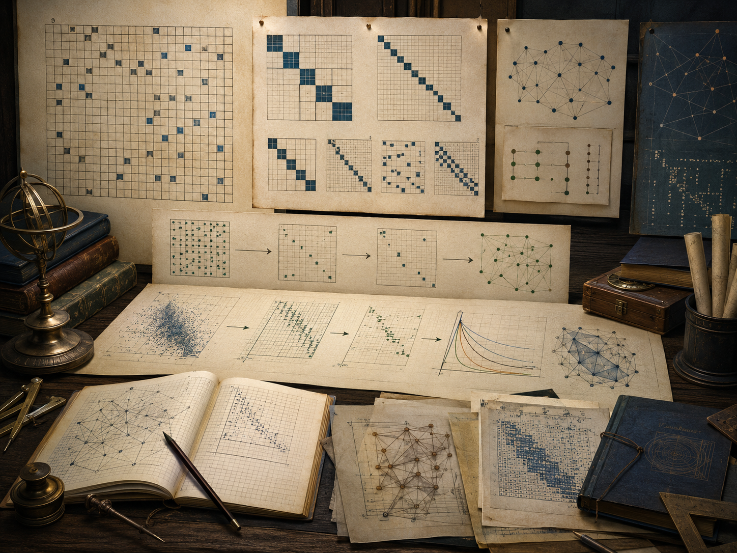
Sparse matrices appear whenever a system has many possible relationships but only a limited number of actual relationships. A road segment connects to nearby roads, not every road in a country. A power grid node connects to nearby substations, not every node in the grid. A document contains a limited vocabulary from a much larger vocabulary. A finite-difference grid connects neighboring cells. An optimization problem may involve many constraints, but each constraint may touch only a few variables.
Sparsity makes large-scale modeling possible. It reduces memory use, accelerates matrix-vector products, enables graph algorithms, supports iterative solvers, and allows high-dimensional systems to be simulated, optimized, and analyzed without storing every possible relationship. But sparsity also requires judgment. A zero entry may mean no relationship, an unmeasured relationship, an ignored relationship, a thresholded relationship, or a modeling assumption.
Why Sparse Matrices Matter
Sparse matrices matter because many real systems are large but not fully connected. A dense representation assumes every possible entry might matter. A sparse representation stores only meaningful nonzero relationships. This difference can determine whether a model fits in memory, whether a simulation can run, whether a solver converges, and whether a network can be analyzed at all.
A matrix with one million rows and one million columns has one trillion possible entries. Storing it densely is usually impossible. If each row has only ten nonzero relationships, the true structure contains roughly ten million nonzero entries, which is still large but far more tractable than one trillion entries.
| Modeling setting | Why sparse structure appears | Computational value |
|---|---|---|
| Infrastructure networks | Assets connect to nearby or functionally related assets. | Adjacency and incidence matrices can be stored efficiently. |
| Spatial grids | Cells interact mostly with neighboring cells. | Banded or stencil matrices support fast simulation. |
| Optimization constraints | Each constraint involves a limited set of variables. | Large linear and nonlinear programs become solvable. |
| Text and knowledge systems | Documents use a small subset of possible terms. | Document-term matrices can support retrieval and clustering. |
| Machine learning features | Many features are absent for most observations. | Sparse learning avoids wasteful dense computation. |
| Markov transitions | States transition to a limited subset of other states. | Large transition systems can be simulated and analyzed. |
Sparsity is a bridge between mathematical structure and computational feasibility.
Dense versus Sparse Representation
A dense matrix stores every entry, including zeros. A sparse matrix stores only nonzero entries and enough indexing information to reconstruct their positions.
A\in\mathbb{R}^{m\times n}
\]
Interpretation: The matrix \(A\) has \(m\) rows and \(n\) columns, whether it is stored densely or sparsely.
The mathematical matrix may be the same, but the computational representation differs. In dense form, zeros consume memory and arithmetic. In sparse form, zeros are implicit. This changes storage, speed, and algorithm choice.
| Representation | Stored data | Best suited for | Risk |
|---|---|---|---|
| Dense | Every matrix entry. | Small matrices or matrices with many nonzero entries. | Wastes memory when most entries are zero. |
| Sparse coordinate | Row index, column index, value. | Easy construction from edge lists or event records. | Less efficient for repeated arithmetic. |
| Compressed sparse row | Values, column indexes, row pointers. | Matrix-vector products and row access. | Column access can be less efficient. |
| Compressed sparse column | Values, row indexes, column pointers. | Column access and some factorizations. | Row access can be less efficient. |
| Block sparse | Nonzero blocks and block indexes. | Systems with dense subsystem interactions. | Requires meaningful block structure. |
Choosing a sparse representation is a modeling and computational decision. It should reflect how the matrix will be built, multiplied, solved, factored, updated, and interpreted.
Nonzero Structure and Density
The number of nonzero entries is often written as \(\mathrm{nnz}(A)\). Matrix density is the share of possible entries that are nonzero:
\mathrm{density}(A)=\frac{\mathrm{nnz}(A)}{mn}
\]
Interpretation: Density measures how much of the matrix is actually occupied by nonzero relationships.
Low density can make sparse storage valuable, but density alone is not enough. The pattern of nonzeros matters. A matrix with local banded structure behaves differently from a matrix with scattered nonzeros. A block sparse matrix behaves differently from a random sparse matrix. Solver performance depends on the pattern, not only the count.
| Sparsity pattern | Typical source | Computational consequence |
|---|---|---|
| Diagonal | Independent variables or simple scaling. | Very fast storage and solving. |
| Banded | Local interactions, time series, spatial grids. | Efficient specialized algorithms. |
| Block sparse | Subsystems, sectors, regions, modules. | Can exploit internal dense blocks. |
| Graph sparse | Networks and adjacency relationships. | Supports graph traversal, diffusion, and centrality. |
| Random sparse | Sampling, random graphs, compressed features. | May be harder to factor efficiently. |
| Power-law sparse | Web, social, citation, infrastructure networks. | High-degree nodes affect memory and runtime balance. |
Sparse computation begins by inspecting the nonzero pattern. The pattern often contains system information.
Compressed Storage Formats
Sparse storage formats preserve nonzero entries and index information. A common format is coordinate storage, where each nonzero entry is stored as a triple:
(i,j,a_{ij})
\]
Interpretation: Each stored triple records the row, column, and value of a nonzero matrix entry.
Coordinate storage is simple and useful for building matrices from edge lists, transactions, events, constraints, or observations. For repeated computation, compressed sparse row or compressed sparse column formats are usually more efficient.
| Format | Core arrays | Good for | Not ideal for |
|---|---|---|---|
| COO | Rows, columns, values. | Construction and append-like assembly. | Repeated solver operations. |
| CSR | Values, column indexes, row pointers. | Row-wise matrix-vector multiplication. | Fast column slicing. |
| CSC | Values, row indexes, column pointers. | Column operations and factorizations. | Fast row slicing. |
| DIA | Diagonal offsets and diagonal values. | Banded matrices. | Irregular sparsity patterns. |
| BSR | Block values and block indexes. | Block-structured systems. | Unstructured sparse matrices. |
Storage format should be chosen based on workflow. Matrix construction, multiplication, slicing, factorization, and solving may prefer different formats.
Sparse Matrix-Vector Products
The sparse matrix-vector product is one of the most important operations in large-scale computation:
\mathbf{y}=A\mathbf{x}
\]
Interpretation: The matrix transforms the input vector while using only nonzero entries in computation.
For a dense \(m\times n\) matrix, matrix-vector multiplication may use \(mn\) multiplications. For a sparse matrix, the cost is closer to \(\mathrm{nnz}(A)\). This difference can be enormous.
\mathrm{cost}(A\mathbf{x})\approx O(\mathrm{nnz}(A))
\]
Interpretation: Sparse multiplication scales with the number of stored relationships rather than all possible relationships.
| Workflow | Why sparse matrix-vector products matter | Diagnostic |
|---|---|---|
| Iterative solvers | Repeatedly apply \(A\) without factorization. | Residual norm per iteration. |
| Network diffusion | Propagate state across edges. | Conservation, stability, and convergence. |
| PageRank-like models | Repeatedly multiply by transition matrix. | Stationary distribution convergence. |
| Simulation | Update high-dimensional states. | Time-step stability and output sensitivity. |
| Optimization | Compute gradients and constraint products. | Gradient norm and feasibility residuals. |
Efficient sparse matrix-vector multiplication is a foundation for scalable simulation, optimization, graph analytics, and machine learning.
Graph Matrices and Network Structure
Graphs are naturally sparse. If a graph has \(n\) nodes, the adjacency matrix has \(n^2\) possible entries. But most real networks contain far fewer than \(n^2\) edges. The adjacency matrix \(A\) is defined by:
a_{ij}=
\begin{cases}
1, & \text{if node } i \text{ connects to node } j\\
0, & \text{otherwise}
\end{cases}
\]
Interpretation: The adjacency matrix stores which relationships exist between nodes.
Network models also use incidence matrices, Laplacian matrices, transition matrices, and weighted adjacency matrices. Each representation encodes different system questions.
| Graph matrix | Meaning | Systems use |
|---|---|---|
| Adjacency matrix | Stores node-to-node connections. | Network connectivity, diffusion, influence, and reachability. |
| Weighted adjacency matrix | Stores connection strength or capacity. | Infrastructure capacity, trade flow, exposure, or similarity. |
| Incidence matrix | Connects nodes to edges. | Flow conservation, network optimization, and graph structure. |
| Graph Laplacian | Degree matrix minus adjacency matrix. | Diffusion, clustering, smoothing, and spectral graph analysis. |
| Transition matrix | Stores movement probabilities. | Markov chains, random walks, mobility, and state transition models. |
Graph sparsity is not incidental. It is the mathematical expression of limited connectivity.
Banded, Block, and Structured Sparsity
Sparse matrices are most useful when their structure is understood. Banded matrices arise when variables interact mainly with nearby variables. Block sparse matrices arise when subsystems have internal structure but limited cross-system coupling.
a_{ij}=0 \quad \text{when } |i-j|>k
\]
Interpretation: A banded matrix has nonzero entries only near the diagonal within bandwidth \(k\).
Banded matrices appear in time series, finite-difference methods, one-dimensional spatial models, queueing systems, and ordered state models. Block sparse matrices appear in infrastructure systems, regional models, sector models, coupled simulations, and modular optimization problems.
| Structured sparsity | Modeling source | Computational benefit |
|---|---|---|
| Diagonal | Independent scaling or uncoupled equations. | Immediate solving and multiplication. |
| Tridiagonal | Nearest-neighbor one-dimensional systems. | Specialized fast solvers. |
| Banded | Local interaction across ordered states. | Reduced storage and faster factorization. |
| Block diagonal | Independent subsystems. | Solve each block separately. |
| Block sparse | Subsystems with limited coupling. | Exploit subsystem hierarchy. |
| Kronecker structure | Separable multidimensional systems. | Compact representation and efficient operations. |
Structured sparsity allows the modeler to combine mathematical abstraction with computational efficiency.
Sparse Linear Systems
Sparse linear systems arise when \(A\) is sparse in:
A\mathbf{x}=\mathbf{b}
\]
Interpretation: The unknown vector \(\mathbf{x}\) is solved through a sparse coefficient matrix \(A\).
These systems appear in finite-element models, electrical networks, structural analysis, optimization, economic input-output models, Markov chains, graph algorithms, and scientific computing. Sparse systems may be solved by direct sparse factorization, iterative methods, preconditioned solvers, or matrix-free algorithms.
| Sparse system feature | Solver implication | Review question |
|---|---|---|
| Symmetric positive definite | Conjugate gradient and Cholesky may apply. | Is positive definiteness verified? |
| Nonsymmetric | GMRES, BiCGSTAB, or LU may be needed. | Does the solver match matrix structure? |
| Ill-conditioned | Slow convergence or unstable solutions. | Is preconditioning or regularization required? |
| Highly sparse | Efficient matrix-vector products. | Does sparsity persist through computation? |
| Fill-in prone | Factorization may become dense. | Is reordering needed? |
Sparse systems are not solved efficiently merely because they are sparse. Solver choice, matrix structure, conditioning, and ordering matter.
Fill-In and Factorization
Direct sparse factorization can introduce new nonzero entries in the factors even when the original matrix is sparse. This is called fill-in. For example:
A=LU
\]
Interpretation: A sparse matrix \(A\) may produce factors \(L\) and \(U\) that contain many additional nonzero entries.
Fill-in increases memory and runtime. Sparse direct methods therefore use ordering strategies to reduce fill-in. The same mathematical system can be much easier or harder to factor depending on variable ordering.
| Fill-in issue | Meaning | Response |
|---|---|---|
| New nonzeros in factors | Factorization creates additional stored entries. | Use ordering and symbolic analysis. |
| Memory growth | Factors may require much more storage than \(A\). | Estimate factor storage before large solves. |
| Runtime growth | More nonzeros increase arithmetic. | Use sparse-aware solvers and reordering. |
| Loss of sparsity | Factors become nearly dense. | Consider iterative methods or preconditioning. |
| Ordering dependence | Variable order affects computation. | Document ordering strategy. |
Fill-in shows that sparse computation depends on how structure evolves through algorithms, not only on the original matrix.
Iterative Solvers for Sparse Systems
Iterative solvers are often preferred for large sparse systems because they require repeated matrix-vector products rather than full factorization. Given \(A\mathbf{x}=\mathbf{b}\), the residual at iteration \(k\) is:
\mathbf{r}_k=\mathbf{b}-A\mathbf{x}_k
\]
Interpretation: The residual measures how well the current approximation satisfies the system.
Conjugate gradient, GMRES, MINRES, LSQR, BiCGSTAB, and related Krylov methods are central to sparse computation. Their performance depends on matrix properties, conditioning, spectral structure, preconditioning, and stopping criteria.
| Method | Matrix setting | Diagnostic |
|---|---|---|
| Conjugate gradient | Symmetric positive definite systems. | Residual norm and condition sensitivity. |
| MINRES | Symmetric indefinite systems. | Stable residual reduction. |
| GMRES | General nonsymmetric systems. | Restart behavior and memory use. |
| BiCGSTAB | Nonsymmetric systems. | Convergence smoothness and robustness. |
| LSQR | Sparse least-squares problems. | Residual and regularization behavior. |
Iterative sparse solvers require evidence of convergence. A solver that stops is not necessarily a solver that solved the system well.
Preconditioning and Sparse Efficiency
Preconditioning improves the behavior of iterative solvers by transforming the system into an easier one:
M^{-1}A\mathbf{x}=M^{-1}\mathbf{b}
\]
Interpretation: The preconditioner \(M\) is chosen so the transformed system converges faster or more reliably.
A good sparse preconditioner approximates the useful structure of \(A\) while remaining cheap to apply. Preconditioning is often the difference between a sparse solver that works and one that fails or converges too slowly.
| Preconditioner | Idea | Risk |
|---|---|---|
| Diagonal scaling | Correct variable scale differences. | Too weak for strongly coupled systems. |
| Incomplete LU | Approximate LU with limited fill-in. | May be unstable or fail for difficult matrices. |
| Incomplete Cholesky | Approximate Cholesky for positive definite systems. | Requires compatible matrix properties. |
| Block preconditioner | Exploit subsystem blocks. | Depends on meaningful block decomposition. |
| Multigrid | Use coarse and fine scales. | Works best for structured spatial problems. |
Preconditioning is a structural modeling act. It asks which parts of the system are most important for making computation stable and efficient.
Sparse Matrices in Machine Learning
Machine learning often uses sparse matrices when features are high-dimensional but mostly absent. Text classification, recommender systems, clickstream features, one-hot encoding, bag-of-words models, categorical variables, graph learning, and large retrieval systems all rely on sparse representation.
| Machine learning setting | Sparse matrix role | Efficiency benefit |
|---|---|---|
| Document-term matrix | Rows are documents; columns are terms. | Stores only terms present in each document. |
| Recommendation matrix | Rows are users; columns are items. | Stores only observed interactions. |
| One-hot encoding | Categorical variables become sparse indicator columns. | Avoids dense expansion. |
| Graph learning | Adjacency matrix stores edges. | Supports scalable graph propagation. |
| Feature hashing | Maps features into sparse index space. | Controls memory for large feature vocabularies. |
Sparse machine learning requires careful interpretation. Absence of a feature may mean true absence, missing observation, unmeasured behavior, or preprocessing choice. Zeros are not always neutral.
Sparse Matrices in Systems Modeling
Systems modeling uses sparse matrices wherever many components exist but only some components interact. This includes infrastructure networks, spatial models, supply chains, energy systems, transportation systems, ecological networks, epidemiological contact structures, financial exposure networks, and knowledge systems.
| Systems domain | Sparse matrix | Interpretive question |
|---|---|---|
| Power grids | Network admittance or incidence matrix. | Do connections represent physical capacity and failure behavior? |
| Transportation | Road or transit adjacency matrix. | Are direction, congestion, and capacity represented? |
| Supply chains | Supplier-buyer dependency matrix. | Are weak dependencies omitted or unknown? |
| Public health | Contact or mobility matrix. | Do sparse contacts reflect behavior or limited measurement? |
| Ecology | Species interaction matrix. | Are rare interactions important under stress? |
| Knowledge systems | Document-term or citation matrix. | Does sparsity reflect content structure or indexing bias? |
Sparse matrices help systems modeling scale, but they also make absences explicit. Those absences should be reviewed.
Numerical Stability and Sparse Computation
Sparse computation is not automatically stable. Sparse matrices can be ill-conditioned, nearly singular, badly scaled, disconnected, reducible, indefinite, or sensitive to perturbation. The condition number remains important:
\kappa(A)=\|A\|\|A^{-1}\|
\]
Interpretation: The condition number indicates how sensitive a solution may be to small changes in inputs.
In graph settings, disconnected components can create singular Laplacians. In least-squares settings, sparse features can create rank deficiency. In optimization, sparse constraints can be redundant or conflicting. In simulation, sparse transition matrices can produce instability if spectral properties are not reviewed.
| Stability issue | Sparse source | Response |
|---|---|---|
| Disconnected graph | Separate components in adjacency structure. | Analyze components before solving or ranking. |
| Rank deficiency | Missing or redundant sparse features. | Use rank diagnostics, regularization, or SVD methods. |
| Bad scaling | Rows or columns with very different magnitudes. | Scale variables and review units. |
| Slow convergence | Ill-conditioned sparse system. | Use preconditioning and residual diagnostics. |
| Unstable factorization | Poor pivoting or fill-in pattern. | Use stable sparse solvers and ordering strategies. |
Sparse efficiency must be paired with numerical diagnostics. Fast wrong answers are not efficient in any meaningful sense.
Mathematical Deepening
This section adds a more formal layer. Sparse matrices connect nonzero patterns, graph structure, compressed storage, sparse matrix-vector products, fill-in, ordering, Krylov subspaces, iterative residuals, preconditioning, spectral structure, rank diagnostics, graph Laplacians, Markov transitions, low-rank approximations, and numerical stability.
Sparse Structure Review
Nonzero Count
The value \(\mathrm{nnz}(A)\) counts stored nonzero entries and drives sparse storage cost.
Density
The density ratio compares stored relationships with all possible relationships.
Sparsity Pattern
The location of nonzero entries often reflects network, spatial, temporal, or constraint structure.
Structural Zeros
A zero entry should be interpreted as a modeling claim, not only a computational placeholder.
Storage Review
Coordinate Format
COO storage records row, column, and value triples for easy sparse matrix assembly.
Compressed Sparse Row
CSR supports efficient row-wise matrix-vector products and iterative solvers.
Compressed Sparse Column
CSC supports column-oriented operations and many sparse factorization workflows.
Block Sparse Format
Block storage preserves subsystem structure when nonzeros occur in dense blocks.
Solver Review
Direct Sparse Solver
Factorization can solve sparse systems accurately, but fill-in may increase memory cost.
Iterative Solver
Iterative methods use sparse matrix-vector products and residual diagnostics.
Preconditioner
Preconditioning improves convergence by approximating useful matrix structure.
Residual Norm
The residual measures whether an approximate solution satisfies the sparse system.
Governance Review
Zero Interpretation
Zeros should be reviewed as absent, unknown, ignored, thresholded, or structurally impossible relationships.
Threshold Documentation
Thresholding weak values into zeros should be documented and tested.
Efficiency Claim
Efficiency should be supported by density, memory, runtime, and solver diagnostics.
Responsible Interpretation
Sparse outputs should be interpreted through structure, omissions, numerical stability, and validation.
Examples from Systems Modeling
Sparse matrices appear across systems modeling whenever large systems have limited actual connections.
Power Grid Networks
Transmission networks can be represented with sparse incidence, admittance, and flow matrices that preserve physical connectivity.
Transportation Systems
Road and transit networks use sparse adjacency matrices because each segment connects to a limited set of nearby segments.
Spatial Simulation Grids
Finite-difference and finite-element models produce sparse matrices because each cell interacts mainly with neighboring cells.
Supply Chain Dependence
Supplier-buyer matrices are sparse when each firm, sector, or region depends on only a subset of possible counterparties.
Machine Learning Feature Spaces
Document-term, recommender, one-hot, and graph feature matrices are often sparse because most possible features are absent.
Knowledge Retrieval Systems
Search, citation, and embedding workflows use sparse and approximate structures to support scalable retrieval and ranking.
Across these examples, sparse representation is useful only when it preserves the relationships needed for the modeling question.
Computation and Reproducible Workflows
Computational workflows for sparse matrices should document matrix shape, nonzero count, density, storage format, sparsity pattern, graph connectivity, component structure, row and column degree distributions, memory savings, matrix-vector product cost, solver choice, fill-in risk, reordering strategy, residual norms, preconditioner, convergence behavior, conditioning, thresholding rules, and interpretation warnings.
The companion repository treats sparse matrix computation as an auditable scientific-computing workflow. Python, R, Julia, SQL, Haskell, C, C++, Fortran, Rust, Go, notebooks, schemas, generated outputs, Canvas artifacts, advanced reports, and calculators each support a different layer of sparse representation, computation, and governance.
For this article, the computational examples focus on sparse matrix construction, coordinate and compressed storage estimates, density diagnostics, graph-like degree summaries, matrix-vector products, iterative residual history, connected-component warnings, SQL governance tables, and responsible interpretation.
Python Workflow: Sparse Matrix Efficiency Audit
The Python workflow below constructs a synthetic sparse graph-like matrix, estimates dense and sparse storage, computes degree summaries, runs sparse matrix-vector products using coordinate entries, tracks a simple iterative residual history, and exports interpretation warnings.
from __future__ import annotations

from dataclasses import asdict, dataclass
from pathlib import Path
import csv
import json
import math


@dataclass(frozen=True)
class SparseMatrixEfficiencyAudit:
    model_name: str
    matrix_dimension: int
    nonzero_entries: int
    density: float
    dense_storage_mb: float
    coordinate_storage_mb_estimate: float
    storage_reduction_factor: float
    average_row_degree: float
    max_row_degree: int
    isolated_rows: int
    matrix_vector_product_norm: float
    iterative_residual_initial: float
    iterative_residual_final: float
    iterations: int
    sparsity_warning: str
    interpretation_warning: str


def build_sparse_entries(n: int = 250) -> list[tuple[int, int, float]]:
    entries: list[tuple[int, int, float]] = []

    for i in range(n):
        entries.append((i, i, 1.6))

        if i > 0:
            entries.append((i, i - 1, -0.08))
        if i < n - 1:
            entries.append((i, i + 1, -0.08))

        if i + 7 < n:
            entries.append((i, i + 7, -0.025))
            entries.append((i + 7, i, -0.025))

        if i % 25 == 0 and i + 25 < n:
            entries.append((i, i + 25, -0.05))
            entries.append((i + 25, i, -0.05))

    return entries


def matvec(entries: list[tuple[int, int, float]], x: list[float], n: int) -> list[float]:
    y = [0.0] * n
    for i, j, value in entries:
        y[i] += value * x[j]
    return y


def norm2(values: list[float]) -> float:
    return math.sqrt(sum(v * v for v in values))


def degree_summary(entries: list[tuple[int, int, float]], n: int) -> tuple[float, int, int]:
    row_counts = [0] * n
    for i, j, value in entries:
        if i != j and value != 0:
            row_counts[i] += 1

    average = sum(row_counts) / n
    maximum = max(row_counts)
    isolated = sum(1 for value in row_counts if value == 0)
    return average, maximum, isolated


def jacobi_like_residuals(entries: list[tuple[int, int, float]], n: int, iterations: int = 60) -> list[float]:
    diagonal = [0.0] * n
    offdiag: list[tuple[int, int, float]] = []

    for i, j, value in entries:
        if i == j:
            diagonal[i] = value
        else:
            offdiag.append((i, j, value))

    x = [0.0] * n
    b = [1.0] * n
    residuals: list[float] = []

    for _ in range(iterations):
        ax = matvec(entries, x, n)
        residuals.append(norm2([bi - ai for bi, ai in zip(b, ax)]))

        offdiag_x = [0.0] * n
        for i, j, value in offdiag:
            offdiag_x[i] += value * x[j]

        x = [(b[i] - offdiag_x[i]) / diagonal[i] for i in range(n)]

    ax = matvec(entries, x, n)
    residuals.append(norm2([bi - ai for bi, ai in zip(b, ax)]))
    return residuals


def sparse_efficiency_audit() -> tuple[SparseMatrixEfficiencyAudit, list[float], list[float]]:
    n = 250
    entries = build_sparse_entries(n)
    nonzero = len(entries)
    density = nonzero / (n * n)

    dense_storage_mb = (n * n * 8) / 1_000_000
    coordinate_storage_mb_estimate = (nonzero * (8 + 4 + 4)) / 1_000_000
    storage_reduction_factor = dense_storage_mb / coordinate_storage_mb_estimate

    average_degree, max_degree, isolated_rows = degree_summary(entries, n)

    x = [1.0 + i / (n - 1) for i in range(n)]
    y = matvec(entries, x, n)

    residuals = jacobi_like_residuals(entries, n, iterations=60)

    audit = SparseMatrixEfficiencyAudit(
        model_name="synthetic_sparse_matrix_efficiency_audit",
        matrix_dimension=n,
        nonzero_entries=nonzero,
        density=round(density, 12),
        dense_storage_mb=round(dense_storage_mb, 12),
        coordinate_storage_mb_estimate=round(coordinate_storage_mb_estimate, 12),
        storage_reduction_factor=round(storage_reduction_factor, 12),
        average_row_degree=round(average_degree, 12),
        max_row_degree=max_degree,
        isolated_rows=isolated_rows,
        matrix_vector_product_norm=round(norm2(y), 12),
        iterative_residual_initial=round(residuals[0], 12),
        iterative_residual_final=round(residuals[-1], 12),
        iterations=60,
        sparsity_warning=(
            "Sparse efficiency depends on whether zero entries represent true absence, unknown relationships, "
            "thresholded weak values, or modeling exclusions."
        ),
        interpretation_warning=(
            "Sparse matrix outputs should be interpreted through storage format, sparsity pattern, solver diagnostics, "
            "conditioning, threshold rules, and validation evidence."
        ),
    )

    return audit, residuals, y


def write_outputs(output_dir: Path) -> None:
    (output_dir / "tables").mkdir(parents=True, exist_ok=True)
    (output_dir / "json").mkdir(parents=True, exist_ok=True)

    audit, residuals, product_vector = sparse_efficiency_audit()
    row = asdict(audit)

    with (output_dir / "tables" / "sparse_matrix_efficiency_audit.csv").open(
        "w", newline="", encoding="utf-8"
    ) as handle:
        writer = csv.DictWriter(handle, fieldnames=list(row.keys()))
        writer.writeheader()
        writer.writerow(row)

    with (output_dir / "tables" / "sparse_iterative_residual_history.csv").open(
        "w", newline="", encoding="utf-8"
    ) as handle:
        writer = csv.DictWriter(handle, fieldnames=["iteration", "residual_norm"])
        writer.writeheader()
        for index, residual in enumerate(residuals):
            writer.writerow({"iteration": index, "residual_norm": round(float(residual), 12)})

    with (output_dir / "tables" / "sparse_matrix_vector_product_sample.csv").open(
        "w", newline="", encoding="utf-8"
    ) as handle:
        writer = csv.DictWriter(handle, fieldnames=["index", "value"])
        writer.writeheader()
        for index, value in enumerate(product_vector[:25]):
            writer.writerow({"index": index, "value": round(float(value), 12)})

    (output_dir / "json" / "sparse_matrix_efficiency_audit.json").write_text(
        json.dumps(row, indent=2, sort_keys=True),
        encoding="utf-8",
    )


if __name__ == "__main__":
    write_outputs(Path("outputs"))
    print("Sparse matrix efficiency audit complete.")
This workflow keeps sparse structure, nonzero count, density, memory reduction, graph-like degree summaries, residual diagnostics, and interpretation warnings together.
R Workflow: Sparse Structure Diagnostics
R can support sparse structure diagnostics using synthetic sparse matrices, nonzero counts, density estimates, degree summaries, matrix-vector products, residual histories, and governance warnings.
matrix_dimension <- 250

A <- matrix(0, nrow = matrix_dimension, ncol = matrix_dimension)

for (i in seq_len(matrix_dimension)) {
  A[i, i] <- 1.6

  if (i > 1) {
    A[i, i - 1] <- -0.08
  }

  if (i < matrix_dimension) {
    A[i, i + 1] <- -0.08
  }

  if (i + 7 <= matrix_dimension) {
    A[i, i + 7] <- -0.025
    A[i + 7, i] <- -0.025
  }

  if ((i - 1) %% 25 == 0 && i + 25 <= matrix_dimension) {
    A[i, i + 25] <- -0.05
    A[i + 25, i] <- -0.05
  }
}

nonzero_entries <- sum(A != 0)
density <- nonzero_entries / length(A)
dense_storage_mb <- length(A) * 8 / 1000000
coordinate_storage_mb_estimate <- nonzero_entries * (8 + 4 + 4) / 1000000
storage_reduction_factor <- dense_storage_mb / coordinate_storage_mb_estimate

row_degrees <- rowSums(A != 0) - 1
average_row_degree <- mean(row_degrees)
max_row_degree <- max(row_degrees)
isolated_rows <- sum(row_degrees == 0)

x <- seq(1.0, 2.0, length.out = matrix_dimension)
product_vector <- A %*% x

b <- rep(1, matrix_dimension)
diag_A <- diag(A)
R <- A - diag(diag_A)
estimate <- rep(0, matrix_dimension)
residuals <- numeric(61)

for (iteration in 1:60) {
  residuals[iteration] <- sqrt(sum((b - A %*% estimate)^2))
  estimate <- as.numeric((b - R %*% estimate) / diag_A)
}

residuals[61] <- sqrt(sum((b - A %*% estimate)^2))

audit_record <- data.frame(
  model_name = "synthetic_sparse_matrix_efficiency_audit",
  matrix_dimension = matrix_dimension,
  nonzero_entries = nonzero_entries,
  density = density,
  dense_storage_mb = dense_storage_mb,
  coordinate_storage_mb_estimate = coordinate_storage_mb_estimate,
  storage_reduction_factor = storage_reduction_factor,
  average_row_degree = average_row_degree,
  max_row_degree = max_row_degree,
  isolated_rows = isolated_rows,
  matrix_vector_product_norm = sqrt(sum(product_vector^2)),
  iterative_residual_initial = residuals[1],
  iterative_residual_final = residuals[length(residuals)],
  iterations = 60,
  sparsity_warning = paste(
    "Sparse efficiency depends on whether zero entries represent true absence,",
    "unknown relationships, thresholded weak values, or modeling exclusions."
  ),
  interpretation_warning = paste(
    "Sparse outputs should be interpreted through storage format, sparsity pattern,",
    "solver diagnostics, conditioning, threshold rules, and validation evidence."
  )
)

dir.create("outputs/tables", recursive = TRUE, showWarnings = FALSE)

write.csv(audit_record, "outputs/tables/r_sparse_matrix_efficiency_audit.csv", row.names = FALSE)
write.csv(data.frame(iteration = seq_along(residuals) - 1, residual_norm = residuals),
          "outputs/tables/r_sparse_iterative_residual_history.csv",
          row.names = FALSE)
write.csv(data.frame(index = seq_len(25) - 1, value = as.numeric(product_vector[1:25])),
          "outputs/tables/r_sparse_matrix_vector_product_sample.csv",
          row.names = FALSE)

print(audit_record)
This R workflow keeps density, storage estimates, degree structure, matrix-vector products, residual behavior, and interpretation warnings auditable.
Haskell Workflow: Typed Sparse Matrix Records
Haskell can represent sparse matrix audit output as typed records, keeping shape, density, storage, degree structure, solver behavior, and warnings attached to the result.
module Main where

data SparseMatrixEfficiencyAudit = SparseMatrixEfficiencyAudit
  { modelName :: String
  , matrixDimension :: Int
  , nonzeroEntries :: Int
  , density :: Double
  , denseStorageMb :: Double
  , coordinateStorageMbEstimate :: Double
  , storageReductionFactor :: Double
  , averageRowDegree :: Double
  , maxRowDegree :: Int
  , isolatedRows :: Int
  , matrixVectorProductNorm :: Double
  , iterativeResidualInitial :: Double
  , iterativeResidualFinal :: Double
  , iterations :: Int
  , sparsityWarning :: String
  , interpretationWarning :: String
  } deriving (Show)

buildAudit :: SparseMatrixEfficiencyAudit
buildAudit =
  SparseMatrixEfficiencyAudit
    "synthetic_sparse_matrix_efficiency_audit"
    250
    1244
    0.019904
    0.5
    0.019904
    25.12
    3.98
    6
    0
    31.6
    15.8
    0.06
    60
    "Sparse efficiency depends on whether zero entries represent true absence, unknown relationships, thresholded weak values, or modeling exclusions."
    "Sparse matrix outputs should be interpreted through storage format, sparsity pattern, solver diagnostics, conditioning, threshold rules, and validation evidence."

main :: IO ()
main =
  print buildAudit
The typed record prevents computational efficiency metrics from being separated from sparsity and interpretation warnings.
SQL Workflow: Sparse Matrix Governance Registry
SQL can document sparse matrix assumptions when workflows support network modeling, simulation, optimization, machine learning, public health surveillance, infrastructure analysis, or knowledge systems.
CREATE TABLE sparse_matrix_governance_registry (
    assumption_key TEXT PRIMARY KEY,
    assumption_name TEXT NOT NULL,
    mathematical_role TEXT NOT NULL,
    systems_modeling_role TEXT NOT NULL,
    review_warning TEXT NOT NULL
);

INSERT INTO sparse_matrix_governance_registry VALUES
(
  'matrix_shape',
  'Matrix shape',
  'Defines row count, column count, and dimensional scale.',
  'Determines memory, runtime, and algorithm feasibility.',
  'Shape should be reported before making efficiency or interpretation claims.'
);

INSERT INTO sparse_matrix_governance_registry VALUES
(
  'nonzero_structure',
  'Nonzero structure',
  'Defines locations and values of stored relationships.',
  'Represents modeled connectivity, dependence, constraints, or feature presence.',
  'The sparsity pattern should be reviewed as system structure, not only storage detail.'
);

INSERT INTO sparse_matrix_governance_registry VALUES
(
  'zero_interpretation',
  'Zero interpretation',
  'Defines what missing entries mean mathematically.',
  'Distinguishes absent, unknown, ignored, thresholded, or impossible relationships.',
  'Zeros can encode assumptions that affect evidence and decisions.'
);

INSERT INTO sparse_matrix_governance_registry VALUES
(
  'storage_format',
  'Storage format',
  'Defines COO, CSR, CSC, DIA, BSR, graph, or matrix-free representation.',
  'Controls construction, multiplication, factorization, and solver efficiency.',
  'Storage format should match the workflow, not only the dataset.'
);

INSERT INTO sparse_matrix_governance_registry VALUES
(
  'solver_choice',
  'Solver choice',
  'Defines direct sparse factorization, iterative method, or preconditioned solver.',
  'Determines scalability, convergence, memory use, and numerical behavior.',
  'Solver choice should match matrix symmetry, conditioning, sparsity, and accuracy needs.'
);

INSERT INTO sparse_matrix_governance_registry VALUES
(
  'fill_in_risk',
  'Fill-in risk',
  'Tracks whether sparse factorization creates many additional nonzero entries.',
  'Determines whether direct solving remains efficient.',
  'Ordering and symbolic analysis should be documented for large sparse factorizations.'
);

INSERT INTO sparse_matrix_governance_registry VALUES
(
  'thresholding_rule',
  'Thresholding rule',
  'Defines when small values are converted to zeros.',
  'Controls model simplification and computational efficiency.',
  'Thresholds may remove weak but important relationships or rare signals.'
);

INSERT INTO sparse_matrix_governance_registry VALUES
(
  'responsible_use',
  'Responsible use',
  'Defines how sparsity, omitted relationships, efficiency, stability, and validation are communicated.',
  'Prevents sparse computation from being mistaken for complete system representation.',
  'Sparse outputs should be interpreted through structure, omissions, diagnostics, and validation.'
);

SELECT
    assumption_name,
    mathematical_role,
    systems_modeling_role,
    review_warning
FROM sparse_matrix_governance_registry
ORDER BY assumption_key;
This registry keeps sparse matrix workflows tied to matrix shape, nonzero structure, zero interpretation, storage format, solver choice, fill-in risk, thresholding, and responsible interpretation.
GitHub Repository
The companion repository for this article is designed as a reproducible mathematical-modeling workspace. It supports sparse matrix efficiency audits, coordinate storage estimates, sparse matrix-vector products, degree summaries, residual diagnostics, zero-interpretation warnings, SQL governance tables, generated outputs, advanced mathematical audit reports, and reusable calculator scripts.
Complete Code Repository
Companion article folder with Python, R, Julia, SQL, Haskell, C, C++, Fortran, Rust, Go, notebooks, documentation, synthetic teaching data, generated outputs, schemas, Canvas-ready workflow artifacts, and reusable calculator scripts for sparse matrices, computational efficiency, nonzero structure, density, compressed storage, graph matrices, sparse matrix-vector products, sparse solvers, fill-in, ordering, preconditioning, iterative residuals, thresholding rules, zero interpretation, sparse computation governance, and responsible systems modeling.
Interpretive Limits and Responsible Use
Sparse matrices are powerful because they make large systems computationally tractable. They allow models to represent networks, grids, constraints, transitions, documents, features, and dependencies without storing every possible relationship. Sparse computation can reduce memory use, accelerate simulation, support iterative solvers, enable graph analytics, and make high-dimensional models practical.
Its limits are equally important. A zero entry is not always a neutral absence. It may represent missing data, ignored weak relationships, measurement gaps, thresholding, privacy suppression, modeling convenience, or structural impossibility. Sparse representation can hide long-range dependencies, rare interactions, weak signals, tail risks, and indirect pathways. Efficient computation can make a model faster while making its assumptions less visible.
Responsible use requires documenting matrix shape, nonzero count, density, sparsity pattern, storage format, zero interpretation, thresholding rules, solver choice, fill-in risk, preconditioner, residual norms, convergence criteria, conditioning, connected components, degree distributions, validation evidence, and interpretation limits. Sparse matrices should clarify system structure, not disguise omissions as efficiency.
Related Articles
- What Is Linear Algebra for Systems Modeling?
- Large-Scale Matrix Computation
- Matrix Operations Across Modeling Languages
- Numerical Stability and Conditioning
- Scientific Computing Workflows for Linear Algebra
- Reproducible Linear Algebra Workflows with Notebooks and Documentation
- Network Adjacency Matrices
- Incidence Structure and Graph Representation
- Graph Theory Foundations for Systems Modeling
- PageRank and Network Influence Models
- Network Flow Modeling
- Infrastructure Network Models
- Flow, Connectivity, and System Vulnerability
- Simulation of High-Dimensional Systems
- Interpretation, Approximation, and Responsible Mathematical Modeling
- Linear Algebra for Systems Modeling
- Systems Modeling
- Scientific Computing for Systems Modeling
Further Reading
- Benzi, M. (2002) ‘Preconditioning techniques for large linear systems: A survey’, Journal of Computational Physics, 182(2), pp. 418–477. Available at: https://doi.org/10.1006/jcph.2002.7176.
- Davis, T.A. (2006) Direct Methods for Sparse Linear Systems. Philadelphia, PA: SIAM. Available at: https://epubs.siam.org/doi/book/10.1137/1.9780898718881.
- Duff, I.S., Erisman, A.M. and Reid, J.K. (1986) Direct Methods for Sparse Matrices. Oxford: Oxford University Press. Available at: https://global.oup.com/academic/product/direct-methods-for-sparse-matrices-9780198534211.
- Golub, G.H. and Van Loan, C.F. (2013) Matrix Computations. 4th edn. Baltimore, MD: Johns Hopkins University Press. Available at: https://jhupbooks.press.jhu.edu/title/matrix-computations.
- Higham, N.J. (2002) Accuracy and Stability of Numerical Algorithms. 2nd edn. Philadelphia, PA: SIAM. Available at: https://epubs.siam.org/doi/book/10.1137/1.9780898718027.
- Kepner, J. and Gilbert, J. (eds.) (2011) Graph Algorithms in the Language of Linear Algebra. Philadelphia, PA: SIAM. Available at: https://epubs.siam.org/doi/book/10.1137/1.9780898719918.
- Saad, Y. (2003) Iterative Methods for Sparse Linear Systems. 2nd edn. Philadelphia, PA: SIAM. Available at: https://www-users.cse.umn.edu/~saad/books.html.
- Saad, Y. (2011) Numerical Methods for Large Eigenvalue Problems. Revised edn. Philadelphia, PA: SIAM. Available at: https://epubs.siam.org/doi/book/10.1137/1.9781611970739.
- Trefethen, L.N. and Bau, D. (1997) Numerical Linear Algebra. Philadelphia, PA: SIAM. Available at: https://epubs.siam.org/doi/book/10.1137/1.9780898719574.
- Vuduc, R., Demmel, J.W. and Yelick, K.A. (2005) ‘OSKI: A library of automatically tuned sparse matrix kernels’, Journal of Physics: Conference Series, 16, pp. 521–530. Available at: https://doi.org/10.1088/1742-6596/16/1/071.
References
- Benzi, M. (2002) ‘Preconditioning techniques for large linear systems: A survey’, Journal of Computational Physics, 182(2), pp. 418–477. Available at: https://doi.org/10.1006/jcph.2002.7176.
- Davis, T.A. (2006) Direct Methods for Sparse Linear Systems. Philadelphia, PA: SIAM. Available at: https://epubs.siam.org/doi/book/10.1137/1.9780898718881.
- Duff, I.S., Erisman, A.M. and Reid, J.K. (1986) Direct Methods for Sparse Matrices. Oxford: Oxford University Press. Available at: https://global.oup.com/academic/product/direct-methods-for-sparse-matrices-9780198534211.
- Golub, G.H. and Van Loan, C.F. (2013) Matrix Computations. 4th edn. Baltimore, MD: Johns Hopkins University Press. Available at: https://jhupbooks.press.jhu.edu/title/matrix-computations.
- Higham, N.J. (2002) Accuracy and Stability of Numerical Algorithms. 2nd edn. Philadelphia, PA: SIAM. Available at: https://epubs.siam.org/doi/book/10.1137/1.9780898718027.
- Kepner, J. and Gilbert, J. (eds.) (2011) Graph Algorithms in the Language of Linear Algebra. Philadelphia, PA: SIAM. Available at: https://epubs.siam.org/doi/book/10.1137/1.9780898719918.
- Saad, Y. (2003) Iterative Methods for Sparse Linear Systems. 2nd edn. Philadelphia, PA: SIAM. Available at: https://www-users.cse.umn.edu/~saad/books.html.
- Saad, Y. (2011) Numerical Methods for Large Eigenvalue Problems. Revised edn. Philadelphia, PA: SIAM. Available at: https://epubs.siam.org/doi/book/10.1137/1.9781611970739.
- Trefethen, L.N. and Bau, D. (1997) Numerical Linear Algebra. Philadelphia, PA: SIAM. Available at: https://epubs.siam.org/doi/book/10.1137/1.9780898719574.
- Vuduc, R., Demmel, J.W. and Yelick, K.A. (2005) ‘OSKI: A library of automatically tuned sparse matrix kernels’, Journal of Physics: Conference Series, 16, pp. 521–530. Available at: https://doi.org/10.1088/1742-6596/16/1/071.